unbal_nonoverlap_exploration
Annie Xie
2025-04-29
Last updated: 2025-05-05
Checks: 7 0
Knit directory:
symmetric_covariance_decomposition/
This reproducible R Markdown analysis was created with workflowr (version 1.7.1). The Checks tab describes the reproducibility checks that were applied when the results were created. The Past versions tab lists the development history.
Great! Since the R Markdown file has been committed to the Git repository, you know the exact version of the code that produced these results.
Great job! The global environment was empty. Objects defined in the global environment can affect the analysis in your R Markdown file in unknown ways. For reproduciblity it’s best to always run the code in an empty environment.
The command set.seed(20250408) was run prior to running
the code in the R Markdown file. Setting a seed ensures that any results
that rely on randomness, e.g. subsampling or permutations, are
reproducible.
Great job! Recording the operating system, R version, and package versions is critical for reproducibility.
Nice! There were no cached chunks for this analysis, so you can be confident that you successfully produced the results during this run.
Great job! Using relative paths to the files within your workflowr project makes it easier to run your code on other machines.
Great! You are using Git for version control. Tracking code development and connecting the code version to the results is critical for reproducibility.
The results in this page were generated with repository version fce089f. See the Past versions tab to see a history of the changes made to the R Markdown and HTML files.
Note that you need to be careful to ensure that all relevant files for
the analysis have been committed to Git prior to generating the results
(you can use wflow_publish or
wflow_git_commit). workflowr only checks the R Markdown
file, but you know if there are other scripts or data files that it
depends on. Below is the status of the Git repository when the results
were generated:
Ignored files:
    Ignored:    .DS_Store
    Ignored:    .Rhistory
Note that any generated files, e.g. HTML, png, CSS, etc., are not included in this status report because it is ok for generated content to have uncommitted changes.
These are the previous versions of the repository in which changes were
made to the R Markdown
(analysis/unbal_nonoverlap_exploration.Rmd) and HTML
(docs/unbal_nonoverlap_exploration.html) files. If you’ve
configured a remote Git repository (see ?wflow_git_remote),
click on the hyperlinks in the table below to view the files as they
were in that past version.
| File | Version | Author | Date | Message |
|---|---|---|---|---|
| Rmd | fce089f | Annie Xie | 2025-05-05 | Add exploration of unbalanced nonoverlapping example |
Introduction
In this analysis, I explore the unbalanced non-overlapping setting.
Packages and Functions
library(ebnm)
library(pheatmap)
library(ggplot2)
source('code/symebcovmf_functions.R')
source('code/visualization_functions.R')Data Generation
# adapted from Jason's code
# args is a list containing pop_sizes, branch_sds, indiv_sd, n_genes, and seed
sim_star_data <- function(args) {
  set.seed(args$seed)

  n <- sum(args$pop_sizes)
  p <- args$n_genes
  K <- length(args$pop_sizes)

  FF <- matrix(rnorm(K * p, sd = rep(args$branch_sds, each = p)), ncol = K)

  LL <- matrix(0, nrow = n, ncol = K)
  for (k in 1:K) {
    vec <- rep(0, K)
    vec[k] <- 1
    LL[, k] <- rep(vec, times = args$pop_sizes)
  }

  E <- matrix(rnorm(n * p, sd = args$indiv_sd), nrow = n)
  Y <- LL %*% t(FF) + E
  YYt <- (1/p)*tcrossprod(Y)

  return(list(Y = Y, YYt = YYt, LL = LL, FF = FF, K = ncol(LL)))
}
pop_sizes <- c(20,50,30,60)
n_genes <- 1000
branch_sds <- rep(2,4)
indiv_sd <- 1
seed <- 1
sim_args = list(pop_sizes = pop_sizes, branch_sds = branch_sds, indiv_sd = indiv_sd, n_genes = n_genes, seed = seed)
sim_data <- sim_star_data(sim_args)This is a heatmap of the scaled Gram matrix:
plot_heatmap(sim_data$YYt, colors_range = c('blue','gray96','red'), brks = seq(-max(abs(sim_data$YYt)), max(abs(sim_data$YYt)), length.out = 50))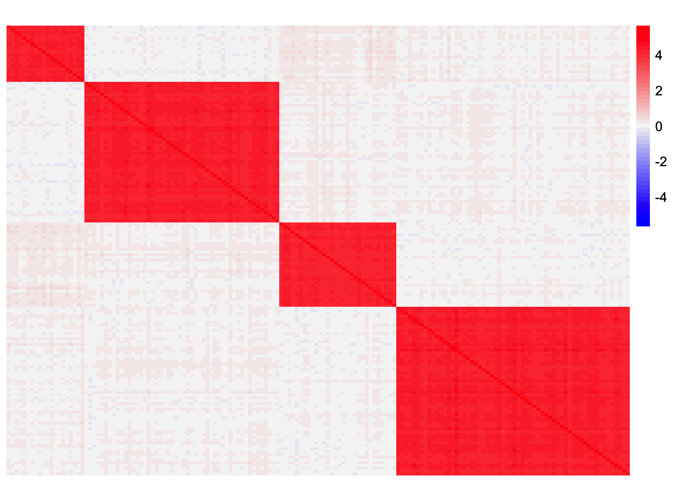
This is a scatter plot of the true loadings matrix:
pop_vec <- rep(c('A','B','C','D'), times = pop_sizes)
plot_loadings(sim_data$LL, pop_vec)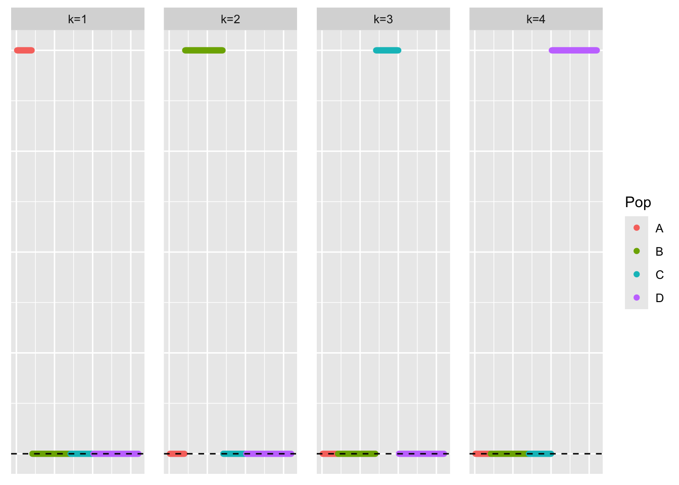
symEBcovMF with refitting
symebcovmf_unbal_refit_fit <- sym_ebcovmf_fit(S = sim_data$YYt, ebnm_fn = ebnm_point_exponential, K = 4, maxiter = 100, rank_one_tol = 10^(-8), tol = 10^(-8), refit_lam = TRUE)Visualization of Estimate
This is a scatter plot of \(\hat{L}_{refit}\), the estimate from symEBcovMF:
plot_loadings(symebcovmf_unbal_refit_fit$L_pm %*% diag(sqrt(symebcovmf_unbal_refit_fit$lambda)), pop_vec)
This is the objective function value attained:
symebcovmf_unbal_refit_fit$elbo[1] 1097.095Visualization of Fit
This is a heatmap of \(\hat{L}_{refit}\hat{\Lambda}_{refit}\hat{L}_{refit}'\):
symebcovmf_unbal_refit_fitted_vals <- tcrossprod(symebcovmf_unbal_refit_fit$L_pm %*% diag(sqrt(symebcovmf_unbal_refit_fit$lambda)))
plot_heatmap(symebcovmf_unbal_refit_fitted_vals, brks = seq(0, max(symebcovmf_unbal_refit_fitted_vals), length.out = 50))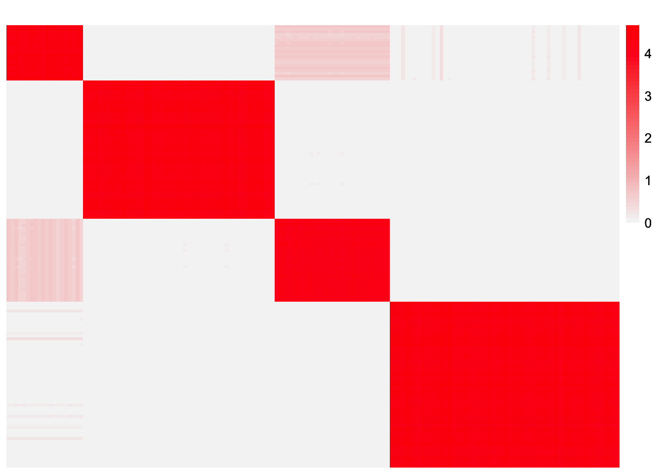
This is a scatter plot of fitted values vs. observed values for the off-diagonal entries:
diag_idx <- seq(1, prod(dim(sim_data$YYt)), length.out = ncol(sim_data$YYt))
off_diag_idx <- setdiff(c(1:prod(dim(sim_data$YYt))), diag_idx)

ggplot(data = NULL, aes(x = c(sim_data$YYt)[off_diag_idx], y = c(symebcovmf_unbal_refit_fitted_vals)[off_diag_idx])) + geom_point() + ylim(-1, 5) + xlim(-1,5) + xlab('Observed Values') + ylab('Fitted Values') + geom_abline(slope = 1, intercept = 0, color = 'red')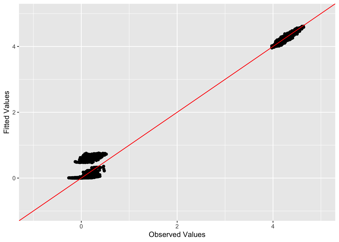
Observations
As noted in a different analysis, symEBcovMF does a relatively good job at recovering the four population effects. However, one undesired aspect of the estimate is that factor 3 contains the effects of two different groups. I would like to figure out why this is happening. Furthermore, the group 1 effect is much smaller than the group 4 effect, so I’m wondering if it’s possible to shrink the group 1 effect down to zero so that the factor only captures one group.
Trying a smaller convergence tolerance
In this section, we explore whether a smaller convergence tolerance will yield a factor which captures only one group. Perhaps the group 1 effect is in the process of being (slowly) shrunk down to zero, and a smaller tolerance will allow for more shrinkage.
symebcovmf_unbal_refit_smaller_tol_fit <- sym_ebcovmf_fit(S = sim_data$YYt, ebnm_fn = ebnm_point_exponential, K = 4, maxiter = 100, rank_one_tol = 10^(-15), tol = 10^(-8), refit_lam = TRUE)[1] "elbo decreased by 7.27595761418343e-12"
[1] "elbo decreased by 1.45519152283669e-11"
[1] "elbo decreased by 1.2732925824821e-11"
[1] "elbo decreased by 1.90993887372315e-11"Visualization of Estimate
This is a scatter plot of \(\hat{L}_{refit}\), the estimate from symEBcovMF:
plot_loadings(symebcovmf_unbal_refit_smaller_tol_fit$L_pm %*% diag(sqrt(symebcovmf_unbal_refit_smaller_tol_fit$lambda)), pop_vec)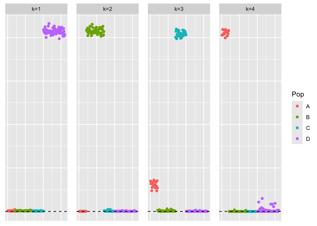
This is the objective function value attained:
symebcovmf_unbal_refit_smaller_tol_fit$elbo[1] 1097.121Comparison of factor 3 estimates:
ggplot(data = NULL, aes(x = symebcovmf_unbal_refit_fit$L_pm[,3], y = symebcovmf_unbal_refit_smaller_tol_fit$L_pm[,3])) + geom_point() + geom_abline(slope = 1, intercept = 0, color = 'red')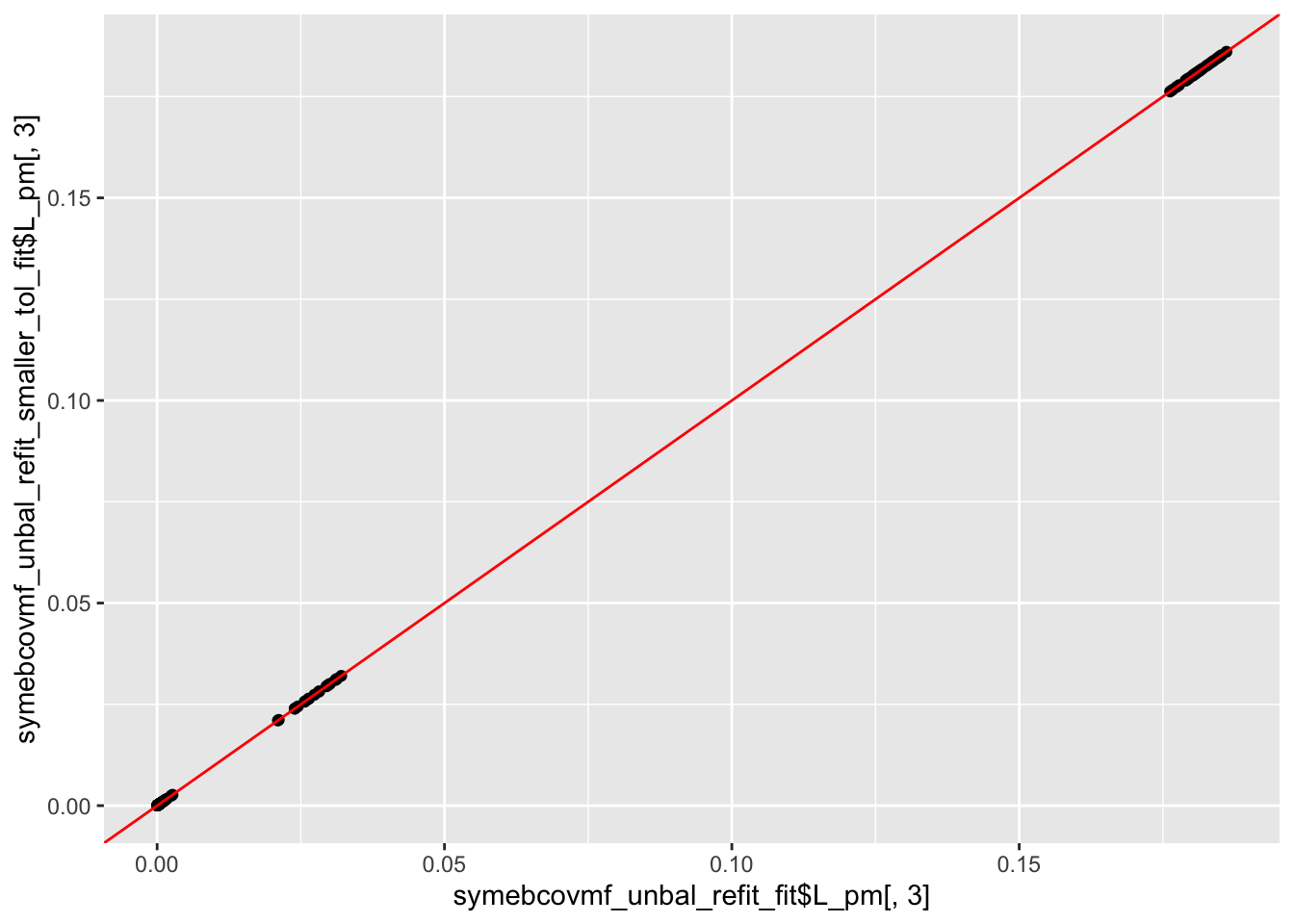
Observations
Decreasing the convergence tolerance does not lead to more shrinkage of the group 1 effect in the factor 3 estimate. The optimization procedure for factor 3 does stop because the ELBO slightly decreases (on the order of \(10^{-11}\)). My guess is the decrease is caused by a numerical issue. So it’s possible that we would see more shrinkage if we let the optimization run for more iterations.
Try initializing from true factor
To check if this is a convergence issue, I try fitting the third factor initialized from the true single population effect factor.
First, we fit the first two factors.
symebcovmf_unbal_refit_rank2_fit <- sym_ebcovmf_fit(S = sim_data$YYt, ebnm_fn = ebnm_point_exponential, K = 2, maxiter = 100, rank_one_tol = 10^(-8), tol = 10^(-8), refit_lam = TRUE)This is a heatmap of the residual matrix, \(S - \sum_{k=1}^{2} \hat{\lambda}_k \hat{\ell}_k \hat{\ell}_k'\):
R <- sim_data$YYt - tcrossprod(symebcovmf_unbal_refit_rank2_fit$L_pm %*% diag(sqrt(symebcovmf_unbal_refit_rank2_fit$lambda)))
plot_heatmap(R, colors_range = c('blue','gray96','red'), brks = seq(-max(abs(R)), max(abs(R)), length.out = 50))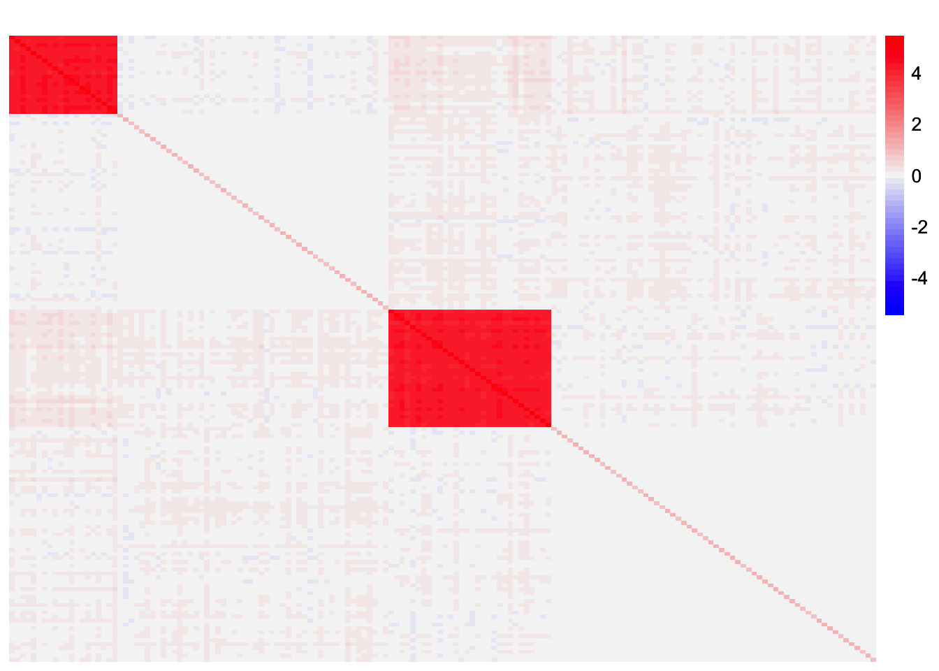
Now, we fit the third factor, initialized with the true population effect factor.
symebcovmf_unbal_true_init_fac3_fit <- sym_ebcovmf_r1_fit(S = sim_data$YYt, symebcovmf_unbal_refit_rank2_fit, ebnm_fn = ebnm::ebnm_point_exponential, maxiter = 100, tol = 10^(-8), v_init = rep(c(0,0,1,0), times = pop_sizes))This is a plot of the estimate of the third factor.
plot(symebcovmf_unbal_true_init_fac3_fit$L_pm[,3], ylab = 'Third Factor')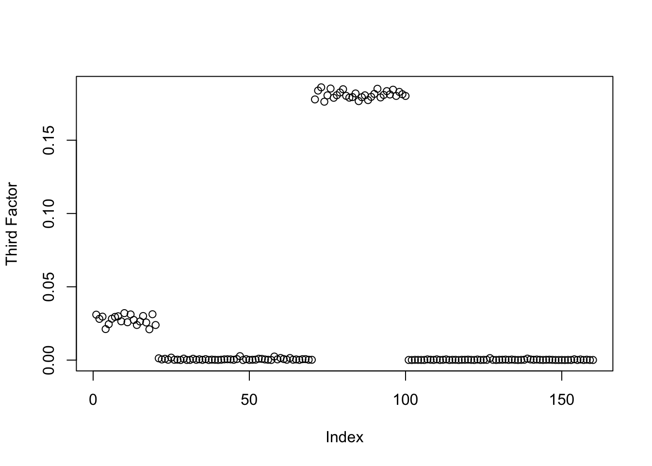
This is a plot of the ELBO during the fit of the third factor.
fac3.idx <- which(symebcovmf_unbal_true_init_fac3_fit$vec_elbo_full == 3)
plot(symebcovmf_unbal_true_init_fac3_fit$vec_elbo_full[(fac3.idx+1):length(symebcovmf_unbal_true_init_fac3_fit$vec_elbo_full)], ylab = 'ELBO')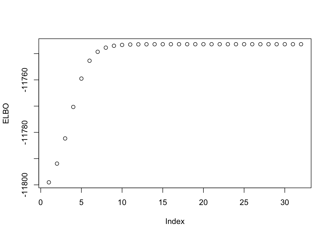
true_fac3 <- rep(c(0,0,1,0), times = pop_sizes)
true_fac3 <- true_fac3/sqrt(sum(true_fac3^2))
estimates_list <- list(true_fac3)
for (i in 1:11){
  estimates_list[[(i+1)]] <- sym_ebcovmf_r1_fit(sim_data$YYt, symebcovmf_unbal_refit_rank2_fit, ebnm_fn = ebnm::ebnm_point_exponential, maxiter = i, tol = 10^(-8), v_init = rep(c(0,0,1,0), times = pop_sizes))$L_pm[,3]
}
This is a plot of the progression of the estimate.
par(mfrow = c(6,2), mar = c(2, 2, 1, 1) + 0.1)
max_y <- max(sapply(estimates_list, max))
min_y <- min(sapply(estimates_list, min))
for (i in 1:12){
  plot(estimates_list[[i]], main = paste('Iter', (i-1)), ylab = 'L', ylim = c(min_y, max_y))
}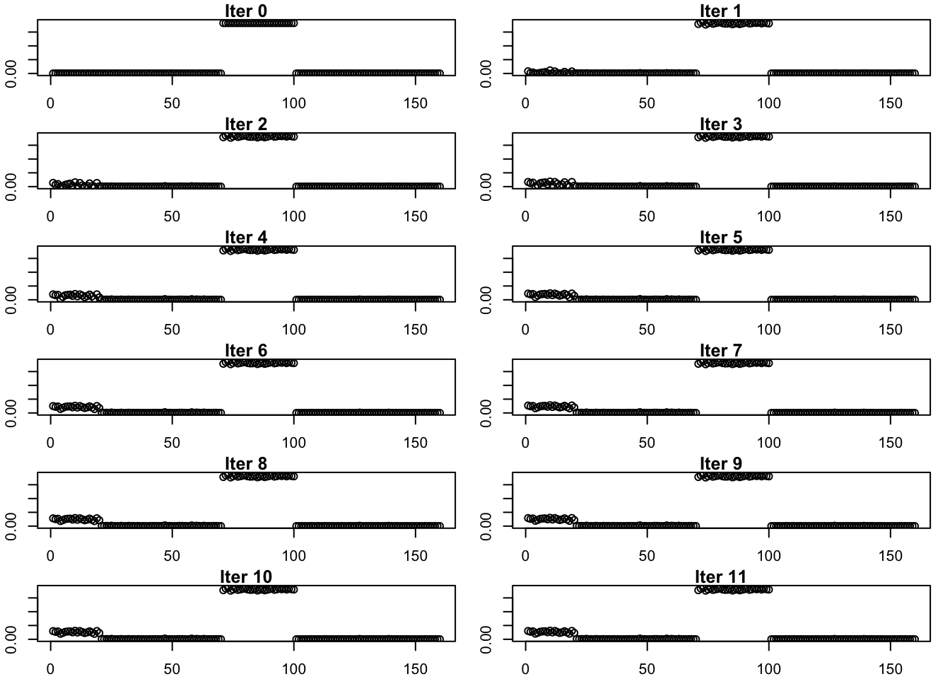
par(mfrow = c(1,1))Observations
When initialized with the true factor, the method still yields an estimate that has non-zero loading on the first group. This suggests that the method does prefer this estimate. Perhaps an easier way of getting a representation comprised of four single group effect factors is to backfit. Question I have: why does this method have this issue but EBMFcov-greedy does not?
sessionInfo()R version 4.3.2 (2023-10-31)
Platform: aarch64-apple-darwin20 (64-bit)
Running under: macOS Sonoma 14.4.1
Matrix products: default
BLAS: /Library/Frameworks/R.framework/Versions/4.3-arm64/Resources/lib/libRblas.0.dylib
LAPACK: /Library/Frameworks/R.framework/Versions/4.3-arm64/Resources/lib/libRlapack.dylib; LAPACK version 3.11.0
locale:
[1] en_US.UTF-8/en_US.UTF-8/en_US.UTF-8/C/en_US.UTF-8/en_US.UTF-8
time zone: America/Chicago
tzcode source: internal
attached base packages:
[1] stats graphics grDevices utils datasets methods base
other attached packages:
[1] ggplot2_3.5.1 pheatmap_1.0.12 ebnm_1.1-34 workflowr_1.7.1
loaded via a namespace (and not attached):
[1] gtable_0.3.5 xfun_0.48 bslib_0.8.0 processx_3.8.4
[5] lattice_0.22-6 callr_3.7.6 vctrs_0.6.5 tools_4.3.2
[9] ps_1.7.7 generics_0.1.3 tibble_3.2.1 fansi_1.0.6
[13] highr_0.11 pkgconfig_2.0.3 Matrix_1.6-5 SQUAREM_2021.1
[17] RColorBrewer_1.1-3 lifecycle_1.0.4 truncnorm_1.0-9 farver_2.1.2
[21] compiler_4.3.2 stringr_1.5.1 git2r_0.33.0 munsell_0.5.1
[25] getPass_0.2-4 httpuv_1.6.15 htmltools_0.5.8.1 sass_0.4.9
[29] yaml_2.3.10 later_1.3.2 pillar_1.9.0 jquerylib_0.1.4
[33] whisker_0.4.1 cachem_1.1.0 trust_0.1-8 RSpectra_0.16-2
[37] tidyselect_1.2.1 digest_0.6.37 stringi_1.8.4 dplyr_1.1.4
[41] ashr_2.2-66 labeling_0.4.3 splines_4.3.2 rprojroot_2.0.4
[45] fastmap_1.2.0 grid_4.3.2 colorspace_2.1-1 cli_3.6.3
[49] invgamma_1.1 magrittr_2.0.3 utf8_1.2.4 withr_3.0.1
[53] scales_1.3.0 promises_1.3.0 horseshoe_0.2.0 rmarkdown_2.28
[57] httr_1.4.7 deconvolveR_1.2-1 evaluate_1.0.0 knitr_1.48
[61] irlba_2.3.5.1 rlang_1.1.4 Rcpp_1.0.13 mixsqp_0.3-54
[65] glue_1.8.0 rstudioapi_0.16.0 jsonlite_1.8.9 R6_2.5.1
[69] fs_1.6.4