symebcovmf_unbal_nonoverlap
Annie Xie
2025-04-29
Last updated: 2025-05-05
Checks: 7 0
Knit directory:
symmetric_covariance_decomposition/
This reproducible R Markdown analysis was created with workflowr (version 1.7.1). The Checks tab describes the reproducibility checks that were applied when the results were created. The Past versions tab lists the development history.
Great! Since the R Markdown file has been committed to the Git repository, you know the exact version of the code that produced these results.
Great job! The global environment was empty. Objects defined in the global environment can affect the analysis in your R Markdown file in unknown ways. For reproduciblity it’s best to always run the code in an empty environment.
The command set.seed(20250408) was run prior to running
the code in the R Markdown file. Setting a seed ensures that any results
that rely on randomness, e.g. subsampling or permutations, are
reproducible.
Great job! Recording the operating system, R version, and package versions is critical for reproducibility.
Nice! There were no cached chunks for this analysis, so you can be confident that you successfully produced the results during this run.
Great job! Using relative paths to the files within your workflowr project makes it easier to run your code on other machines.
Great! You are using Git for version control. Tracking code development and connecting the code version to the results is critical for reproducibility.
The results in this page were generated with repository version 2e1803a. See the Past versions tab to see a history of the changes made to the R Markdown and HTML files.
Note that you need to be careful to ensure that all relevant files for
the analysis have been committed to Git prior to generating the results
(you can use wflow_publish or
wflow_git_commit). workflowr only checks the R Markdown
file, but you know if there are other scripts or data files that it
depends on. Below is the status of the Git repository when the results
were generated:
Ignored files:
    Ignored:    .DS_Store
    Ignored:    .Rhistory

Untracked files:
    Untracked:  analysis/unbal_nonoverlap_exploration.Rmd
Note that any generated files, e.g. HTML, png, CSS, etc., are not included in this status report because it is ok for generated content to have uncommitted changes.
These are the previous versions of the repository in which changes were
made to the R Markdown (analysis/unbal_nonoverlap.Rmd) and
HTML (docs/unbal_nonoverlap.html) files. If you’ve
configured a remote Git repository (see ?wflow_git_remote),
click on the hyperlinks in the table below to view the files as they
were in that past version.
| File | Version | Author | Date | Message |
|---|---|---|---|---|
| Rmd | 2e1803a | Annie Xie | 2025-05-05 | Update unbalanced nonoverlapping example |
| html | 4ad25a4 | Annie Xie | 2025-04-30 | Build site. |
| Rmd | 28d3567 | Annie Xie | 2025-04-30 | Add analysis of symebcovmf in unbalanced nonoverlapping setting |
Introduction
In this example, we test out symEBcovMF on unbalanced, star-structured data.
Example
library(ebnm)
library(pheatmap)
library(ggplot2)
source('code/symebcovmf_functions.R')
source('code/visualization_functions.R')Data Generation
# adapted from Jason's code
# args is a list containing pop_sizes, branch_sds, indiv_sd, n_genes, and seed
sim_star_data <- function(args) {
  set.seed(args$seed)

  n <- sum(args$pop_sizes)
  p <- args$n_genes
  K <- length(args$pop_sizes)

  FF <- matrix(rnorm(K * p, sd = rep(args$branch_sds, each = p)), ncol = K)

  LL <- matrix(0, nrow = n, ncol = K)
  for (k in 1:K) {
    vec <- rep(0, K)
    vec[k] <- 1
    LL[, k] <- rep(vec, times = args$pop_sizes)
  }

  E <- matrix(rnorm(n * p, sd = args$indiv_sd), nrow = n)
  Y <- LL %*% t(FF) + E
  YYt <- (1/p)*tcrossprod(Y)

  return(list(Y = Y, YYt = YYt, LL = LL, FF = FF, K = ncol(LL)))
}
pop_sizes <- c(20,50,30,60)
n_genes <- 1000
branch_sds <- rep(2,4)
indiv_sd <- 1
seed <- 1
sim_args = list(pop_sizes = pop_sizes, branch_sds = branch_sds, indiv_sd = indiv_sd, n_genes = n_genes, seed = seed)
sim_data <- sim_star_data(sim_args)This is a heatmap of the scaled Gram matrix:
plot_heatmap(sim_data$YYt, colors_range = c('blue','gray96','red'), brks = seq(-max(abs(sim_data$YYt)), max(abs(sim_data$YYt)), length.out = 50))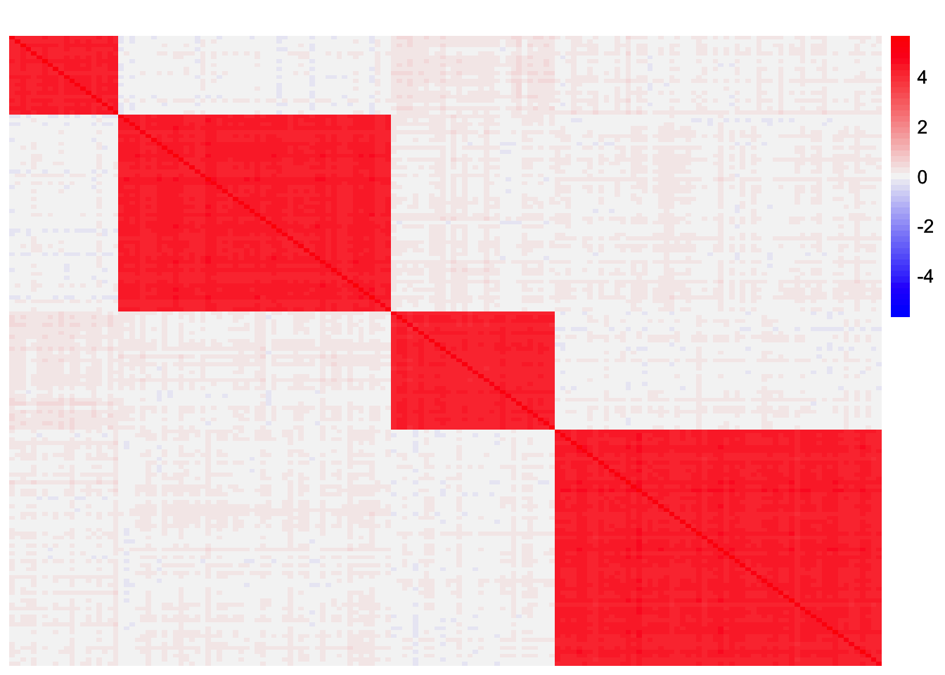
| Version | Author | Date |
|---|---|---|
| 4ad25a4 | Annie Xie | 2025-04-30 |
This is a scatter plot of the true loadings matrix:
pop_vec <- rep(c('A','B','C','D'), times = pop_sizes)
plot_loadings(sim_data$LL, pop_vec)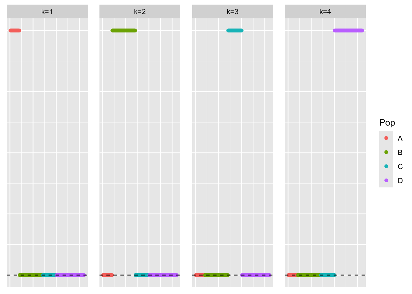
| Version | Author | Date |
|---|---|---|
| 4ad25a4 | Annie Xie | 2025-04-30 |
symEBcovMF
symebcovmf_unbal_fit <- sym_ebcovmf_fit(S = sim_data$YYt, ebnm_fn = ebnm_point_exponential, K = 4, maxiter = 100, rank_one_tol = 10^(-8), tol = 10^(-8))Progression of ELBO
symebcovmf_unbal_full_elbo_vec <- symebcovmf_unbal_fit$vec_elbo_full[!(symebcovmf_unbal_fit$vec_elbo_full %in% c(1:length(symebcovmf_unbal_fit$vec_elbo_K)))]
ggplot() + geom_line(data = NULL, aes(x = 1:length(symebcovmf_unbal_full_elbo_vec), y = symebcovmf_unbal_full_elbo_vec)) + xlab('Iter') + ylab('ELBO')
| Version | Author | Date |
|---|---|---|
| 4ad25a4 | Annie Xie | 2025-04-30 |
Visualization of Estimate
This is a scatter plot of \(\hat{L}\), the estimate from symEBcovMF:
plot_loadings(symebcovmf_unbal_fit$L_pm %*% diag(sqrt(symebcovmf_unbal_fit$lambda)), pop_vec)
| Version | Author | Date |
|---|---|---|
| 4ad25a4 | Annie Xie | 2025-04-30 |
This is the objective function value attained:
symebcovmf_unbal_fit$elbo[1] 1087.677Visualization of Fit
This is a heatmap of \(\hat{L}\hat{\Lambda}\hat{L}'\):
symebcovmf_unbal_fitted_vals <- tcrossprod(symebcovmf_unbal_fit$L_pm %*% diag(sqrt(symebcovmf_unbal_fit$lambda)))
plot_heatmap(symebcovmf_unbal_fitted_vals, brks = seq(0, max(symebcovmf_unbal_fitted_vals), length.out = 50))
| Version | Author | Date |
|---|---|---|
| 4ad25a4 | Annie Xie | 2025-04-30 |
This is a scatter plot of fitted values vs. observed values for the off-diagonal entries:
diag_idx <- seq(1, prod(dim(sim_data$YYt)), length.out = ncol(sim_data$YYt))
off_diag_idx <- setdiff(c(1:prod(dim(sim_data$YYt))), diag_idx)

ggplot(data = NULL, aes(x = c(sim_data$YYt)[off_diag_idx], y = c(symebcovmf_unbal_fitted_vals)[off_diag_idx])) + geom_point() + ylim(-1, 5) + xlim(-1,5) + xlab('Observed Values') + ylab('Fitted Values') + geom_abline(slope = 1, intercept = 0, color = 'red')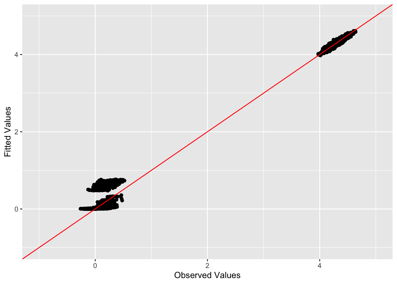
| Version | Author | Date |
|---|---|---|
| 4ad25a4 | Annie Xie | 2025-04-30 |
Observations
symEBcovMF does a relatively good job at recovering the four population effects. Interestingly, while factor 3 primarily recovers the third group effect, it has a small (but still notable) loading on the first group effect. I explore this more in another analysis. I did also try symEBcovMF with generalized binary prior, and in that case, the factors primarily captured one group effect each.
symEBcovMF with refit step
symebcovmf_unbal_refit_fit <- sym_ebcovmf_fit(S = sim_data$YYt, ebnm_fn = ebnm_point_exponential, K = 4, maxiter = 100, rank_one_tol = 10^(-8), tol = 10^(-8), refit_lam = TRUE)Progression of ELBO
symebcovmf_unbal_refit_full_elbo_vec <- symebcovmf_unbal_refit_fit$vec_elbo_full[!(symebcovmf_unbal_refit_fit$vec_elbo_full %in% c(1:length(symebcovmf_unbal_refit_fit$vec_elbo_K)))]
ggplot() + geom_line(data = NULL, aes(x = 1:length(symebcovmf_unbal_refit_full_elbo_vec), y = symebcovmf_unbal_refit_full_elbo_vec)) + xlab('Iter') + ylab('ELBO')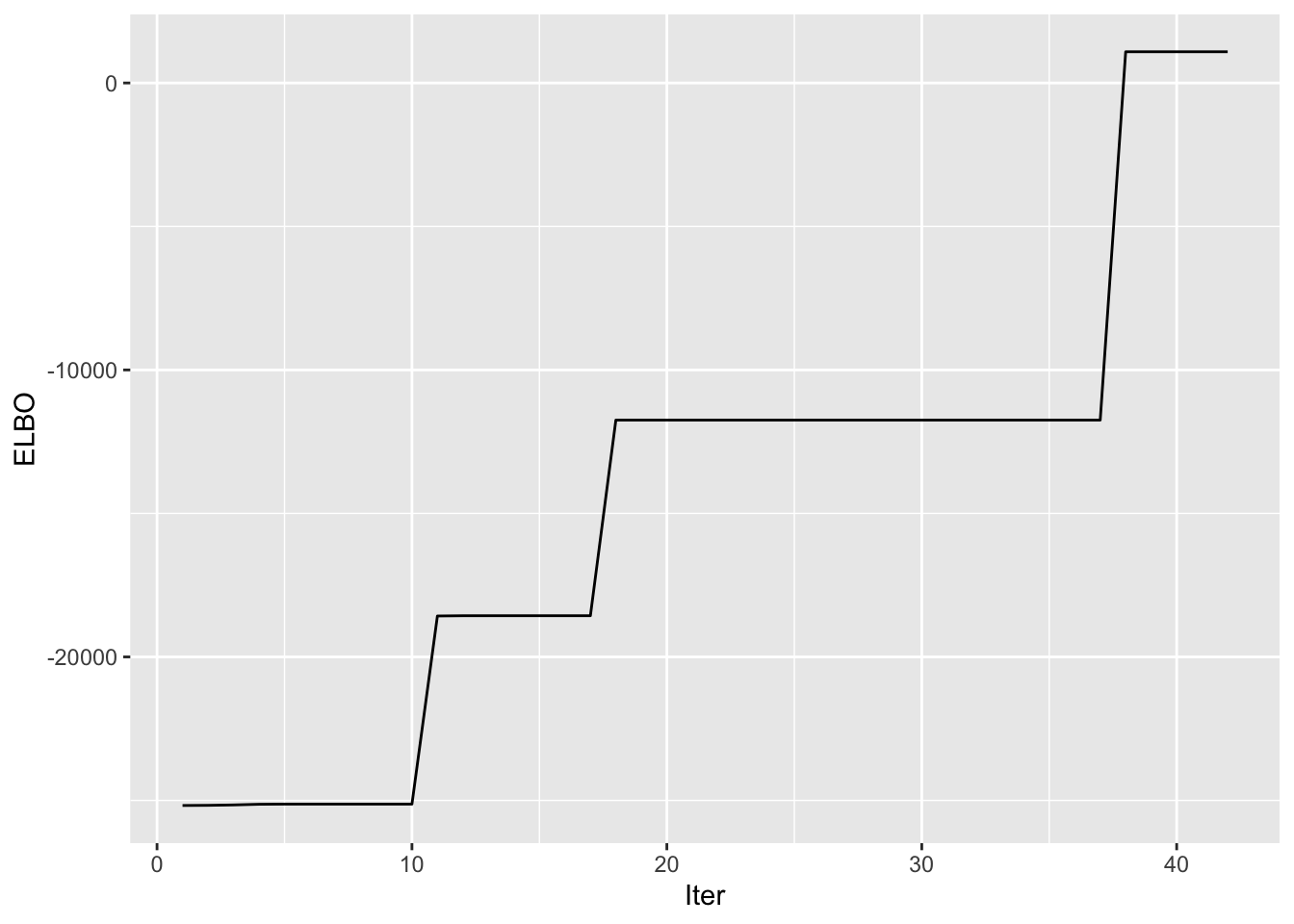
| Version | Author | Date |
|---|---|---|
| 4ad25a4 | Annie Xie | 2025-04-30 |
A note: I don’t think I save the ELBO value after the refitting step in vec_elbo_full. But the refitting does change this vector since it changes the residual matrix that is used when you add a new vector.
Visualization of Estimate
This is a scatter plot of \(\hat{L}_{refit}\), the estimate from symEBcovMF:
plot_loadings(symebcovmf_unbal_refit_fit$L_pm %*% diag(sqrt(symebcovmf_unbal_refit_fit$lambda)), pop_vec)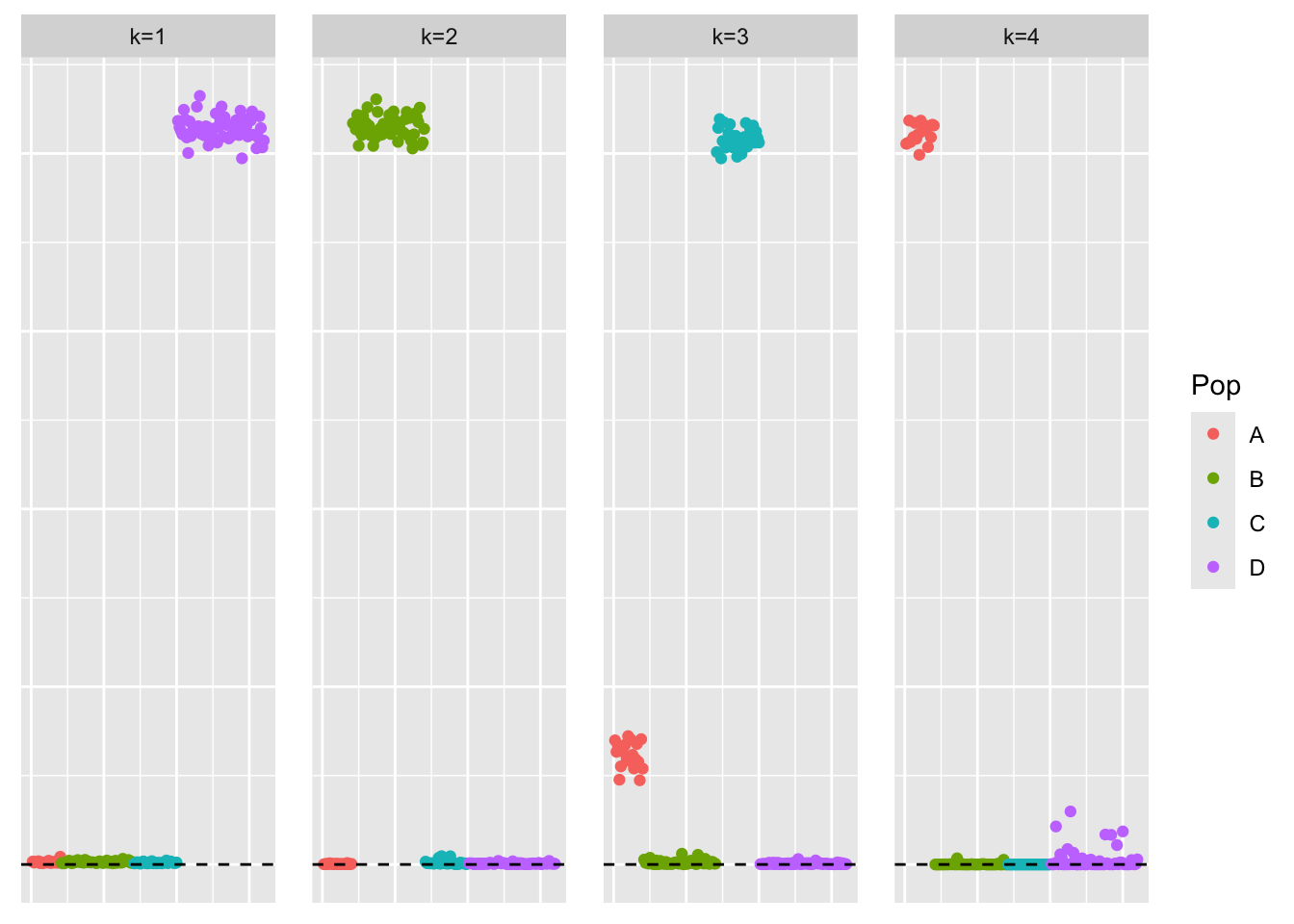
| Version | Author | Date |
|---|---|---|
| 4ad25a4 | Annie Xie | 2025-04-30 |
This is the objective function value attained:
symebcovmf_unbal_refit_fit$elbo[1] 1097.095Visualization of Fit
This is a heatmap of \(\hat{L}_{refit}\hat{\Lambda}_{refit}\hat{L}_{refit}'\):
symebcovmf_unbal_refit_fitted_vals <- tcrossprod(symebcovmf_unbal_refit_fit$L_pm %*% diag(sqrt(symebcovmf_unbal_refit_fit$lambda)))
plot_heatmap(symebcovmf_unbal_refit_fitted_vals, brks = seq(0, max(symebcovmf_unbal_refit_fitted_vals), length.out = 50))
| Version | Author | Date |
|---|---|---|
| 4ad25a4 | Annie Xie | 2025-04-30 |
This is a scatter plot of fitted values vs. observed values for the off-diagonal entries:
diag_idx <- seq(1, prod(dim(sim_data$YYt)), length.out = ncol(sim_data$YYt))
off_diag_idx <- setdiff(c(1:prod(dim(sim_data$YYt))), diag_idx)

ggplot(data = NULL, aes(x = c(sim_data$YYt)[off_diag_idx], y = c(symebcovmf_unbal_refit_fitted_vals)[off_diag_idx])) + geom_point() + ylim(-1, 5) + xlim(-1,5) + xlab('Observed Values') + ylab('Fitted Values') + geom_abline(slope = 1, intercept = 0, color = 'red')
| Version | Author | Date |
|---|---|---|
| 4ad25a4 | Annie Xie | 2025-04-30 |
Comparison of Estimates
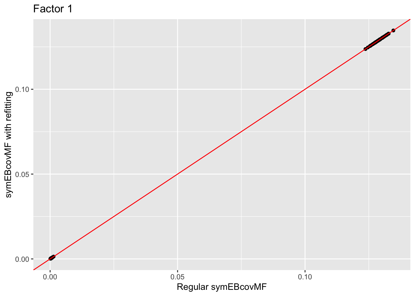
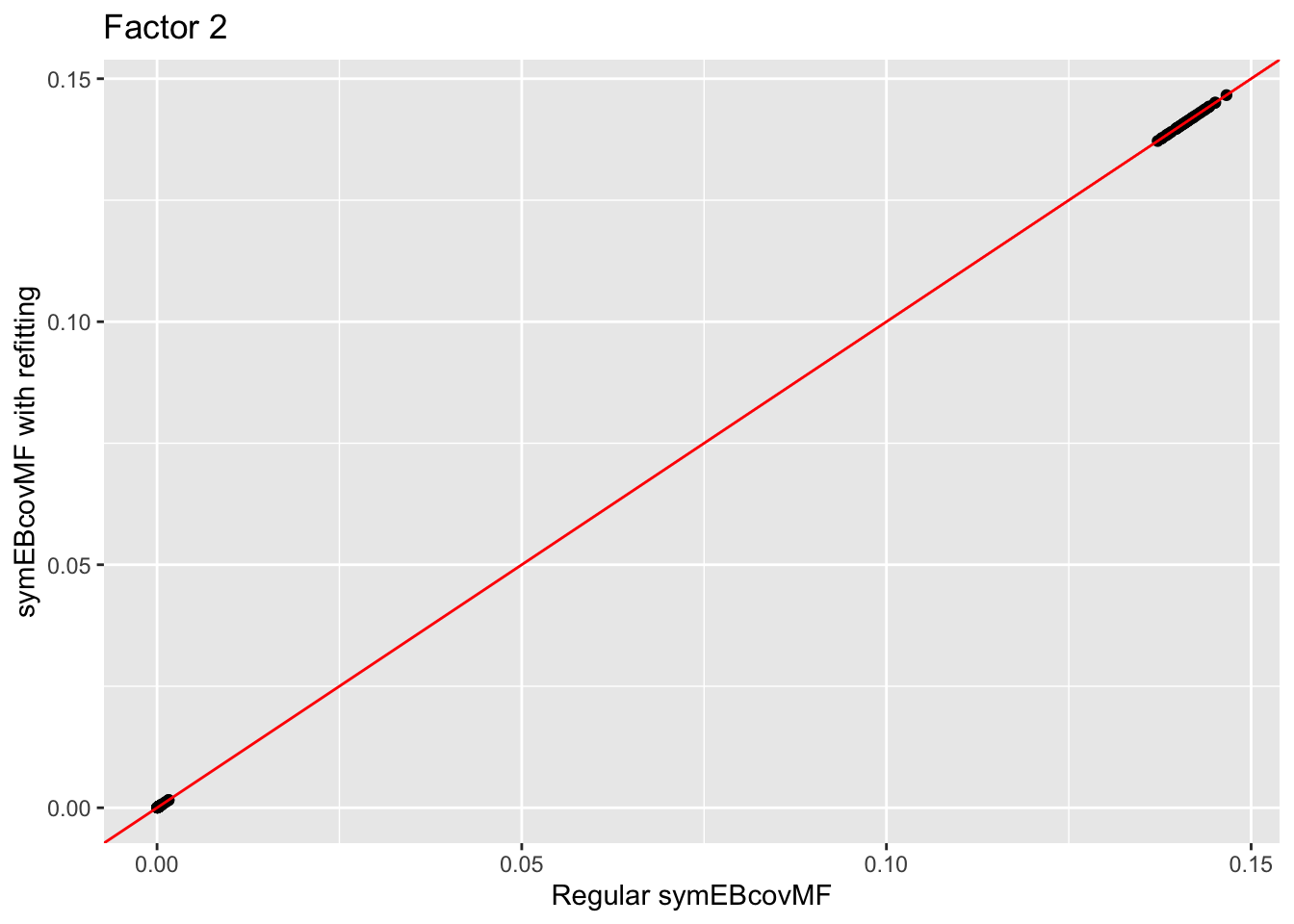
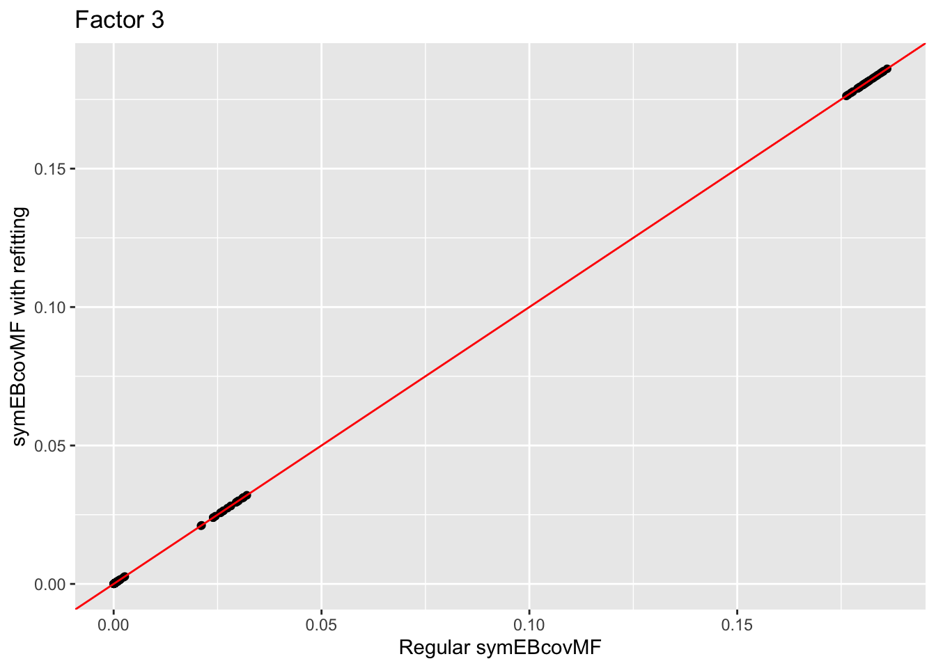
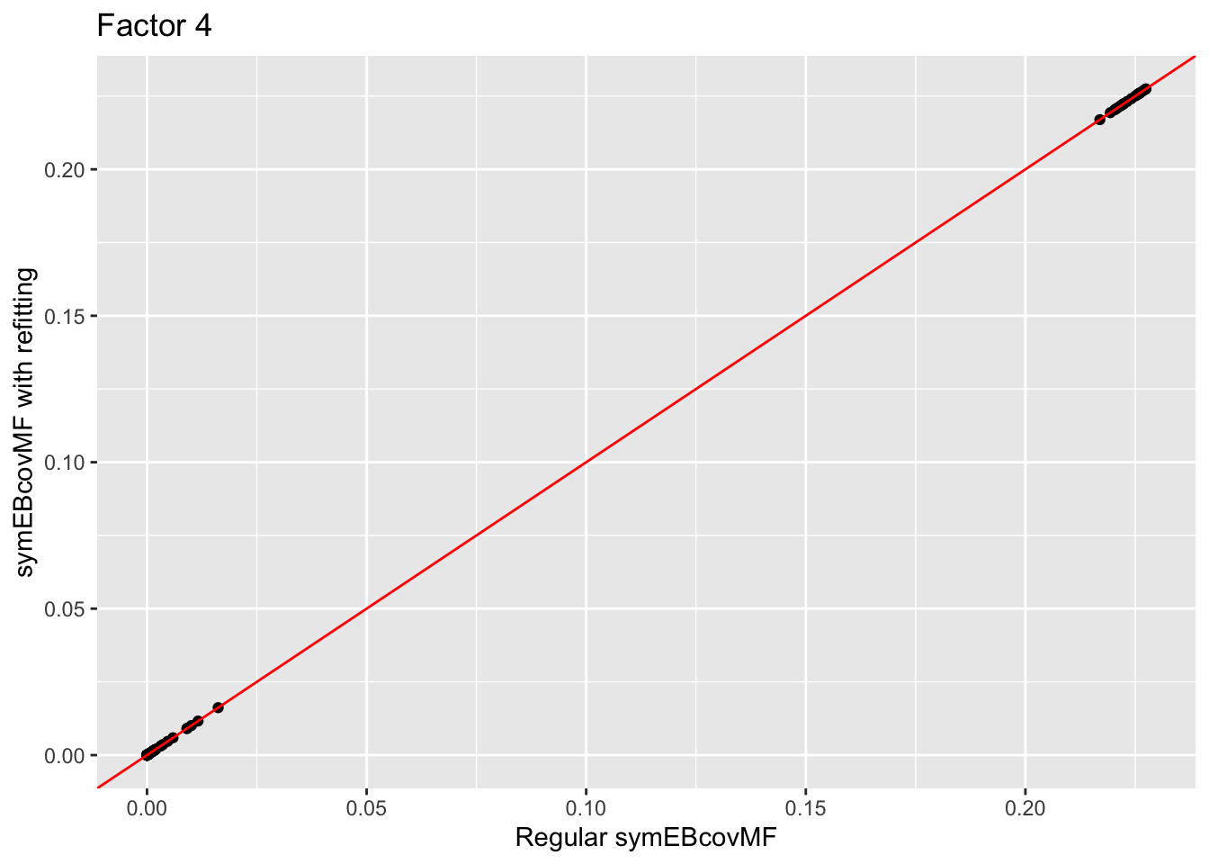
Comparison of the factors:
for (i in 1:4){
  print(ggplot(data = NULL, aes(x = symebcovmf_unbal_fit$L_pm[,i], y = symebcovmf_unbal_refit_fit$L_pm[,i])) + geom_point() + geom_abline(slope = 1, intercept = 0, color = 'red') + ylab('symEBcovMF with refitting') + xlab('Regular symEBcovMF') + labs(title=paste('Factor',i)))
}
| Version | Author | Date |
|---|---|---|
| 4ad25a4 | Annie Xie | 2025-04-30 |
| Version | Author | Date |
|---|---|---|
| 4ad25a4 | Annie Xie | 2025-04-30 |
| Version | Author | Date |
|---|---|---|
| 4ad25a4 | Annie Xie | 2025-04-30 |
| Version | Author | Date |
|---|---|---|
| 4ad25a4 | Annie Xie | 2025-04-30 |
Observations
The estimate from symEBcovMF with refitting qualitatively looks the same as the estimate from regular symEBcovMF. Plotting the values of the two estimates show that they are nearly the same.
sessionInfo()R version 4.3.2 (2023-10-31)
Platform: aarch64-apple-darwin20 (64-bit)
Running under: macOS Sonoma 14.4.1
Matrix products: default
BLAS: /Library/Frameworks/R.framework/Versions/4.3-arm64/Resources/lib/libRblas.0.dylib
LAPACK: /Library/Frameworks/R.framework/Versions/4.3-arm64/Resources/lib/libRlapack.dylib; LAPACK version 3.11.0
locale:
[1] en_US.UTF-8/en_US.UTF-8/en_US.UTF-8/C/en_US.UTF-8/en_US.UTF-8
time zone: America/Chicago
tzcode source: internal
attached base packages:
[1] stats graphics grDevices utils datasets methods base
other attached packages:
[1] ggplot2_3.5.1 pheatmap_1.0.12 ebnm_1.1-34 workflowr_1.7.1
loaded via a namespace (and not attached):
[1] gtable_0.3.5 xfun_0.48 bslib_0.8.0 processx_3.8.4
[5] lattice_0.22-6 callr_3.7.6 vctrs_0.6.5 tools_4.3.2
[9] ps_1.7.7 generics_0.1.3 tibble_3.2.1 fansi_1.0.6
[13] highr_0.11 pkgconfig_2.0.3 Matrix_1.6-5 SQUAREM_2021.1
[17] RColorBrewer_1.1-3 lifecycle_1.0.4 truncnorm_1.0-9 farver_2.1.2
[21] compiler_4.3.2 stringr_1.5.1 git2r_0.33.0 munsell_0.5.1
[25] getPass_0.2-4 httpuv_1.6.15 htmltools_0.5.8.1 sass_0.4.9
[29] yaml_2.3.10 later_1.3.2 pillar_1.9.0 jquerylib_0.1.4
[33] whisker_0.4.1 cachem_1.1.0 trust_0.1-8 RSpectra_0.16-2
[37] tidyselect_1.2.1 digest_0.6.37 stringi_1.8.4 dplyr_1.1.4
[41] ashr_2.2-66 labeling_0.4.3 splines_4.3.2 rprojroot_2.0.4
[45] fastmap_1.2.0 grid_4.3.2 colorspace_2.1-1 cli_3.6.3
[49] invgamma_1.1 magrittr_2.0.3 utf8_1.2.4 withr_3.0.1
[53] scales_1.3.0 promises_1.3.0 horseshoe_0.2.0 rmarkdown_2.28
[57] httr_1.4.7 deconvolveR_1.2-1 evaluate_1.0.0 knitr_1.48
[61] irlba_2.3.5.1 rlang_1.1.4 Rcpp_1.0.13 mixsqp_0.3-54
[65] glue_1.8.0 rstudioapi_0.16.0 jsonlite_1.8.9 R6_2.5.1
[69] fs_1.6.4