symebcovmf_tree_exploration
Annie Xie
2025-04-15
Last updated: 2025-04-21
Checks: 7 0
Knit directory:
symmetric_covariance_decomposition/
This reproducible R Markdown analysis was created with workflowr (version 1.7.1). The Checks tab describes the reproducibility checks that were applied when the results were created. The Past versions tab lists the development history.
Great! Since the R Markdown file has been committed to the Git repository, you know the exact version of the code that produced these results.
Great job! The global environment was empty. Objects defined in the global environment can affect the analysis in your R Markdown file in unknown ways. For reproduciblity it’s best to always run the code in an empty environment.
The command set.seed(20250408) was run prior to running
the code in the R Markdown file. Setting a seed ensures that any results
that rely on randomness, e.g. subsampling or permutations, are
reproducible.
Great job! Recording the operating system, R version, and package versions is critical for reproducibility.
Nice! There were no cached chunks for this analysis, so you can be confident that you successfully produced the results during this run.
Great job! Using relative paths to the files within your workflowr project makes it easier to run your code on other machines.
Great! You are using Git for version control. Tracking code development and connecting the code version to the results is critical for reproducibility.
The results in this page were generated with repository version 1adca4d. See the Past versions tab to see a history of the changes made to the R Markdown and HTML files.
Note that you need to be careful to ensure that all relevant files for
the analysis have been committed to Git prior to generating the results
(you can use wflow_publish or
wflow_git_commit). workflowr only checks the R Markdown
file, but you know if there are other scripts or data files that it
depends on. Below is the status of the Git repository when the results
were generated:
Ignored files:
    Ignored:    .DS_Store
    Ignored:    .Rhistory

Untracked files:
    Untracked:  analysis/symebcovmf_point_exp_init.Rmd
Note that any generated files, e.g. HTML, png, CSS, etc., are not included in this status report because it is ok for generated content to have uncommitted changes.
These are the previous versions of the repository in which changes were
made to the R Markdown
(analysis/symebcovmf_tree_exploration.Rmd) and HTML
(docs/symebcovmf_tree_exploration.html) files. If you’ve
configured a remote Git repository (see ?wflow_git_remote),
click on the hyperlinks in the table below to view the files as they
were in that past version.
| File | Version | Author | Date | Message |
|---|---|---|---|---|
| Rmd | 1adca4d | Annie Xie | 2025-04-21 | Edit source location of visualization functions |
| html | bbe7534 | Annie Xie | 2025-04-21 | Build site. |
| Rmd | 0c0833c | Annie Xie | 2025-04-21 | Add to symebcovmf tree exploration analysis |
| html | a7697e5 | Annie Xie | 2025-04-15 | Build site. |
| Rmd | a41d74d | Annie Xie | 2025-04-15 | Add comparison of priors in tree setting |
Introduction
In this example, we further explore symEBcovMF on tree data.
Packages and Functions
library(ebnm)
library(pheatmap)
library(ggplot2)
source('code/visualization_functions.R')
source('code/symebcovmf_functions.R')Data Generation
sim_4pops <- function(args) {
  set.seed(args$seed)

  n <- sum(args$pop_sizes)
  p <- args$n_genes

  FF <- matrix(rnorm(7 * p, sd = rep(args$branch_sds, each = p)), ncol = 7)
  # if (args$constrain_F) {
  #   FF_svd <- svd(FF)
  #   FF <- FF_svd$u
  #   FF <- t(t(FF) * branch_sds * sqrt(p))
  # }

  LL <- matrix(0, nrow = n, ncol = 7)
  LL[, 1] <- 1
  LL[, 2] <- rep(c(1, 1, 0, 0), times = args$pop_sizes)
  LL[, 3] <- rep(c(0, 0, 1, 1), times = args$pop_sizes)
  LL[, 4] <- rep(c(1, 0, 0, 0), times = args$pop_sizes)
  LL[, 5] <- rep(c(0, 1, 0, 0), times = args$pop_sizes)
  LL[, 6] <- rep(c(0, 0, 1, 0), times = args$pop_sizes)
  LL[, 7] <- rep(c(0, 0, 0, 1), times = args$pop_sizes)

  E <- matrix(rnorm(n * p, sd = args$indiv_sd), nrow = n)
  Y <- LL %*% t(FF) + E
  YYt <- (1/p)*tcrossprod(Y)
  return(list(Y = Y, YYt = YYt, LL = LL, FF = FF, K = ncol(LL)))
}
sim_args = list(pop_sizes = rep(40, 4), n_genes = 1000, branch_sds = rep(2,7), indiv_sd = 1, seed = 1)
sim_data <- sim_4pops(sim_args)This is a heatmap of the scaled Gram matrix:
plot_heatmap(sim_data$YYt, colors_range = c('blue','gray96','red'), brks = seq(-max(abs(sim_data$YYt)), max(abs(sim_data$YYt)), length.out = 50))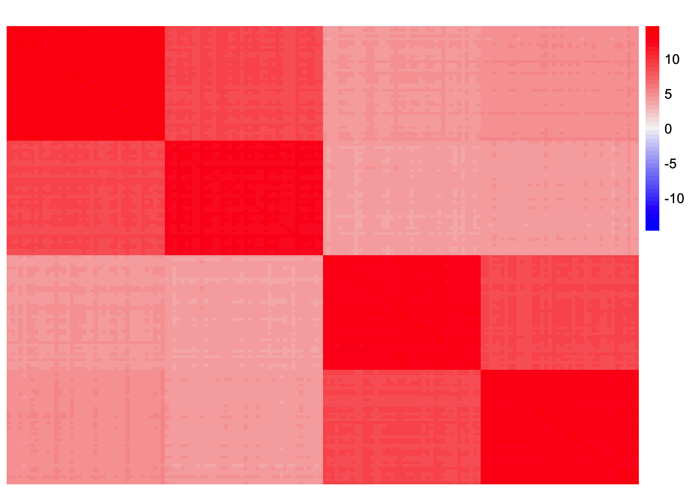
This is a scatter plot of the true loadings matrix:
pop_vec <- c(rep('A', 40), rep('B', 40), rep('C', 40), rep('D', 40))
plot_loadings(sim_data$LL, pop_vec)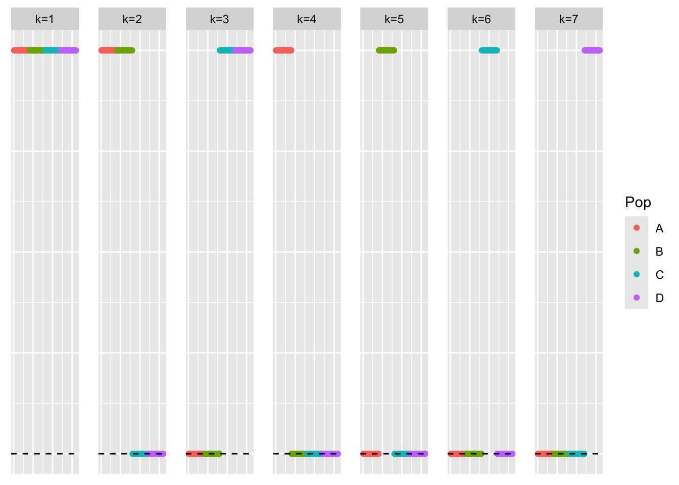
| Version | Author | Date |
|---|---|---|
| a7697e5 | Annie Xie | 2025-04-15 |
This is a plot of the eigenvalues of the Gram matrix:
S_eigen <- eigen(sim_data$YYt)
plot(S_eigen$values) + abline(a = 0, b = 0, col = 'red')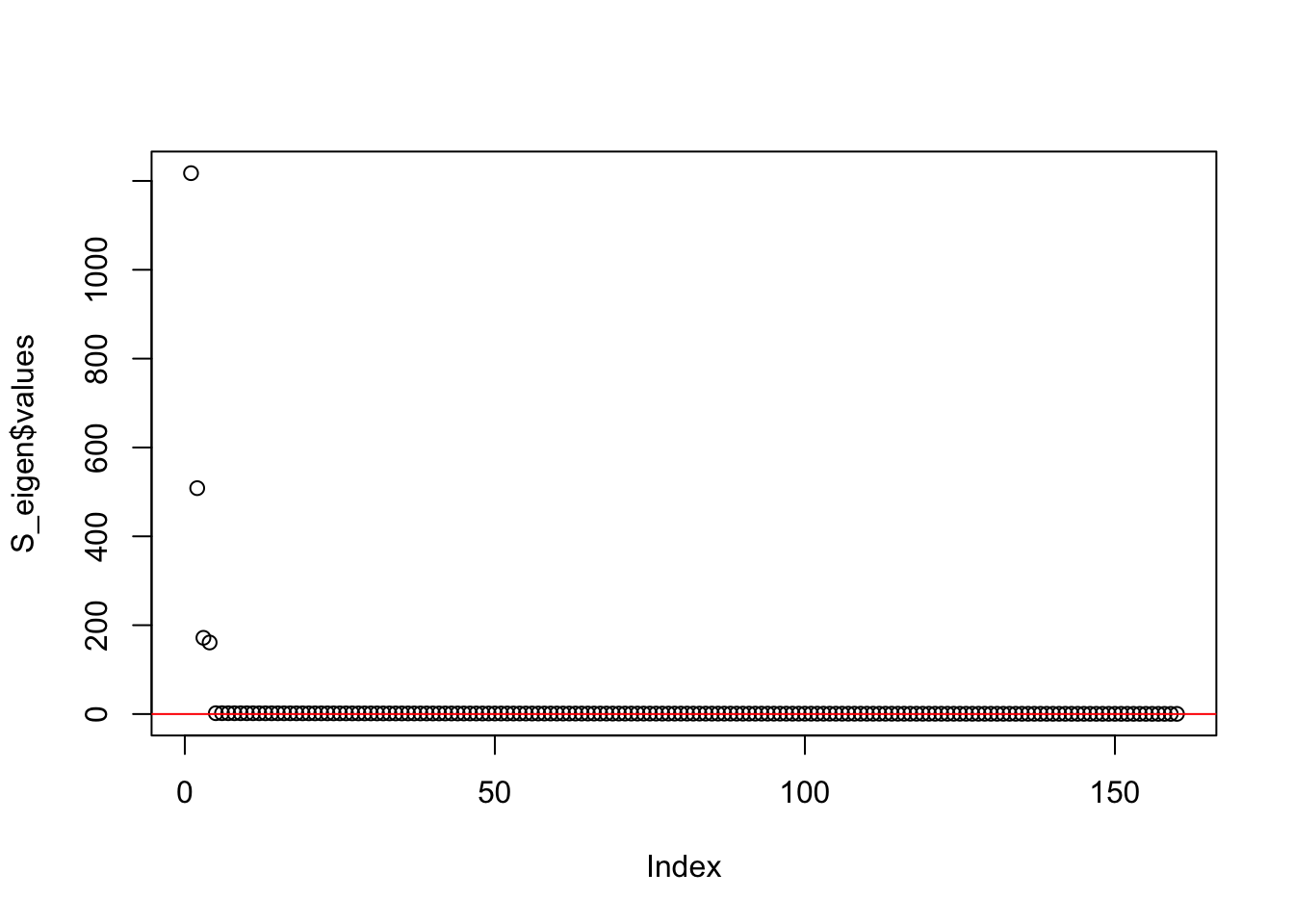
| Version | Author | Date |
|---|---|---|
| a7697e5 | Annie Xie | 2025-04-15 |
integer(0)This is the minimum eigenvalue:
min(S_eigen$values)[1] 0.3724341symEBcovMF Set Up
I am particularly interested in when the fourth factor is fit. So I will start by fitting three factors.
symebcovmf_exp_init_fit <- sym_ebcovmf_fit(S = sim_data$YYt, ebnm_fn = ebnm::ebnm_point_exponential, K = 3, maxiter = 500, rank_one_tol = 10^(-8), tol = 10^(-8), refit_lam = TRUE)symebcovmf_gb_init_fit <- sym_ebcovmf_fit(S = sim_data$YYt, ebnm_fn = ebnm::ebnm_generalized_binary, K = 3, maxiter = 500, rank_one_tol = 10^(-8), tol = 10^(-8), refit_lam = TRUE)[1] "elbo decreased by 0.204520186045556"This is a scatter plot of \(\hat{L}_{exp}\), the estimate from symEBcovMF with point-exp prior:
bal_pops <- c(rep('A', 40), rep('B', 40), rep('C', 40), rep('D', 40))
plot_loadings(symebcovmf_exp_init_fit$L_pm %*% diag(sqrt(symebcovmf_exp_init_fit$lambda)), bal_pops)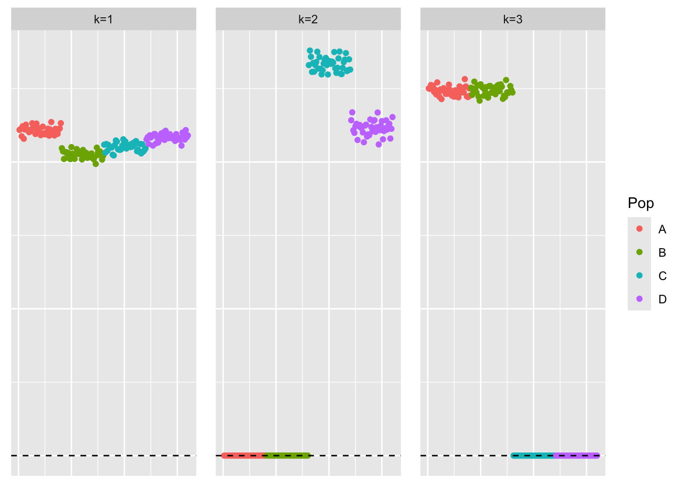
This is a scatter plot of \(\hat{L}_{gb}\), the estimate from symEBcovMF with gb prior:
plot_loadings(symebcovmf_gb_init_fit$L_pm %*% diag(sqrt(symebcovmf_gb_init_fit$lambda)), bal_pops)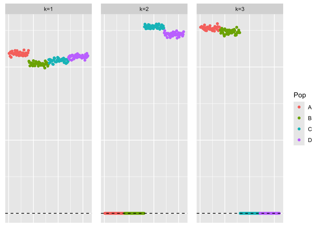
| Version | Author | Date |
|---|---|---|
| a7697e5 | Annie Xie | 2025-04-15 |
This is a plot of the eigenvalues of the residual matrix for point-exp prior:
resid_exp_eigen <- eigen(sim_data$YYt - tcrossprod(symebcovmf_exp_init_fit$L_pm %*% diag(sqrt(symebcovmf_exp_init_fit$lambda), ncol = 1)))
plot(resid_exp_eigen$values) + abline(h=0, col = 'red')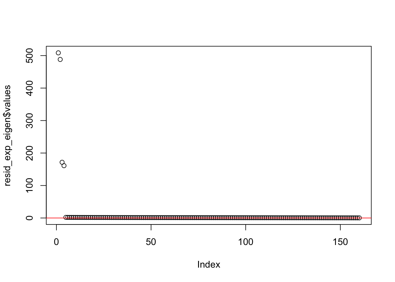
| Version | Author | Date |
|---|---|---|
| a7697e5 | Annie Xie | 2025-04-15 |
integer(0)min(resid_exp_eigen$values)[1] 0.3724341This is a plot of the eigenvalues of the residual matrix for gb prior:
resid_gb_eigen <- eigen(sim_data$YYt - tcrossprod(symebcovmf_gb_init_fit$L_pm %*% diag(sqrt(symebcovmf_gb_init_fit$lambda), ncol = 1)))
plot(resid_gb_eigen$values) + abline(h=0, col = 'red')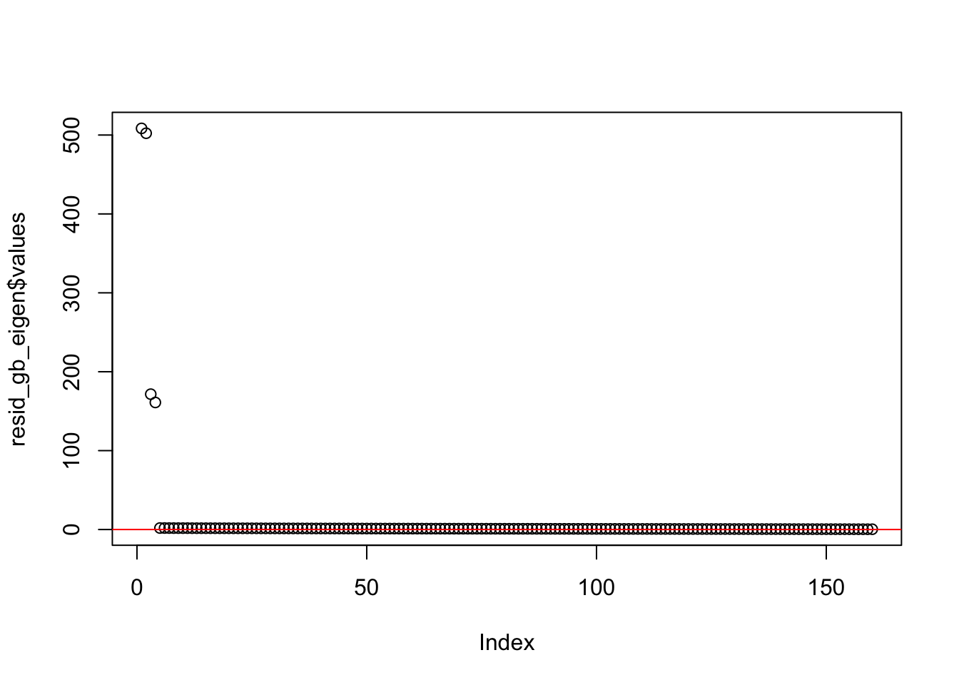
integer(0)min(resid_gb_eigen$values)[1] 0.3724332Fitting the fourth factor
Point-exponential prior
symebcovmf_exp_fit <- sym_ebcovmf_r1_fit(sim_data$YYt, symebcovmf_exp_init_fit, ebnm_fn = ebnm::ebnm_point_exponential, maxiter = 500, tol = 10^(-8))
symebcovmf_exp_fit <- refit_lambda(sim_data$YYt, symebcovmf_exp_fit)
Visualization of Estimate
plot(symebcovmf_exp_fit$L_pm[,4])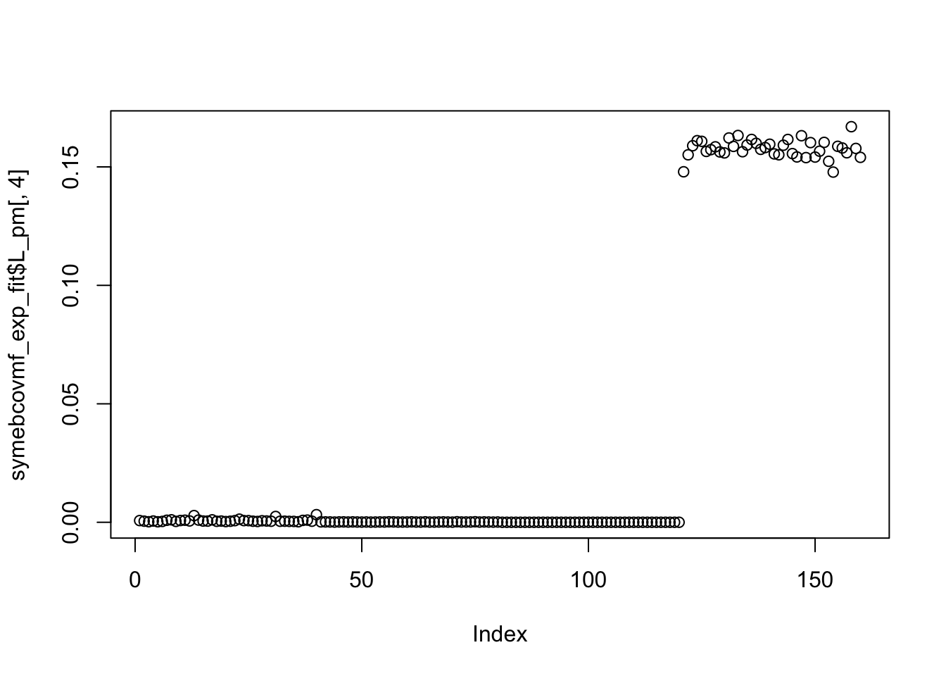
Visualization of ELBO
This is a plot of the progression of the ELBO:
idx <- which(symebcovmf_exp_fit$vec_elbo_full == 4)
plot(symebcovmf_exp_fit$vec_elbo_full[-c(1:idx)], type = 'b', xlab = 'Iter', ylab = 'ELBO') 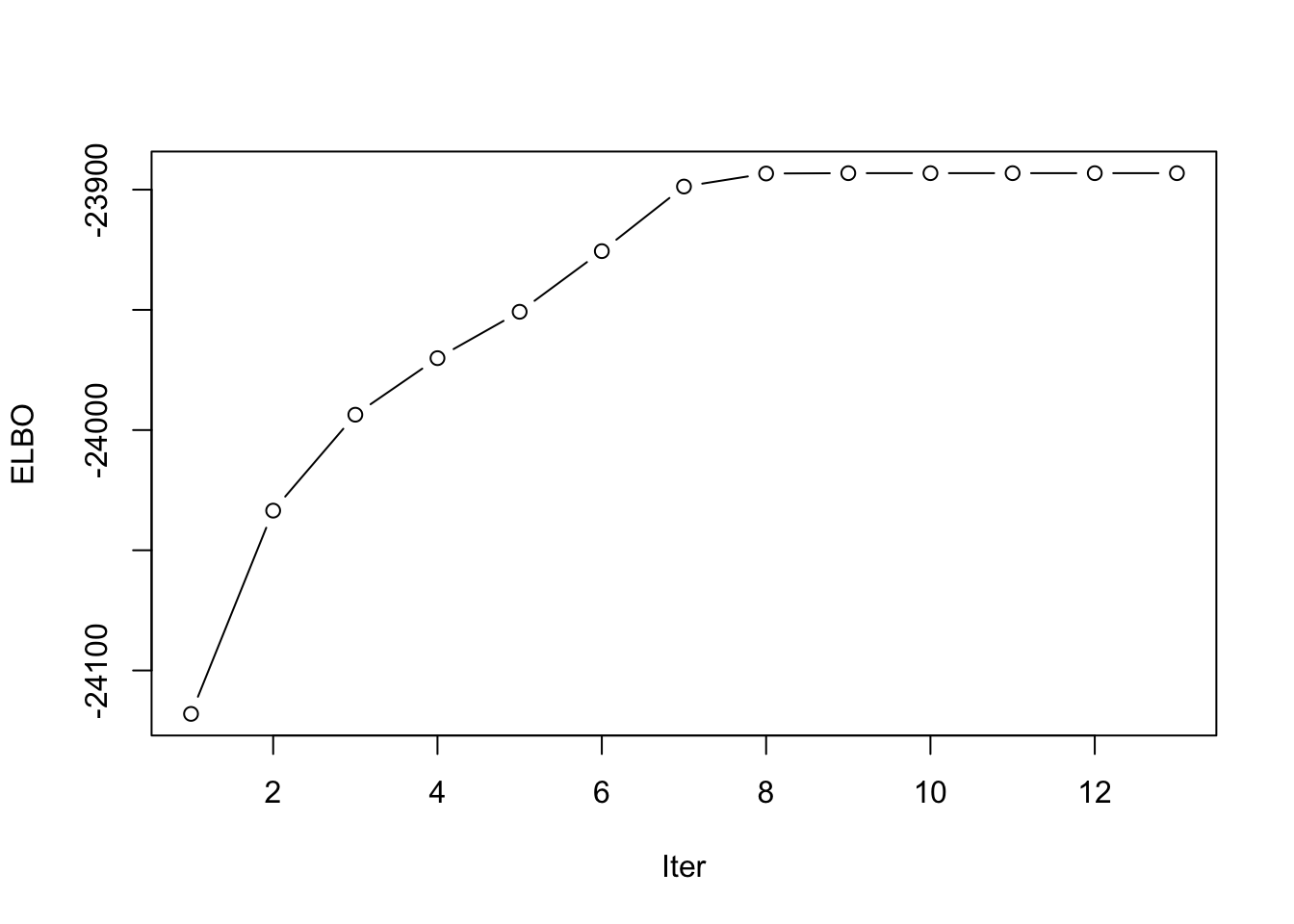
| Version | Author | Date |
|---|---|---|
| a7697e5 | Annie Xie | 2025-04-15 |
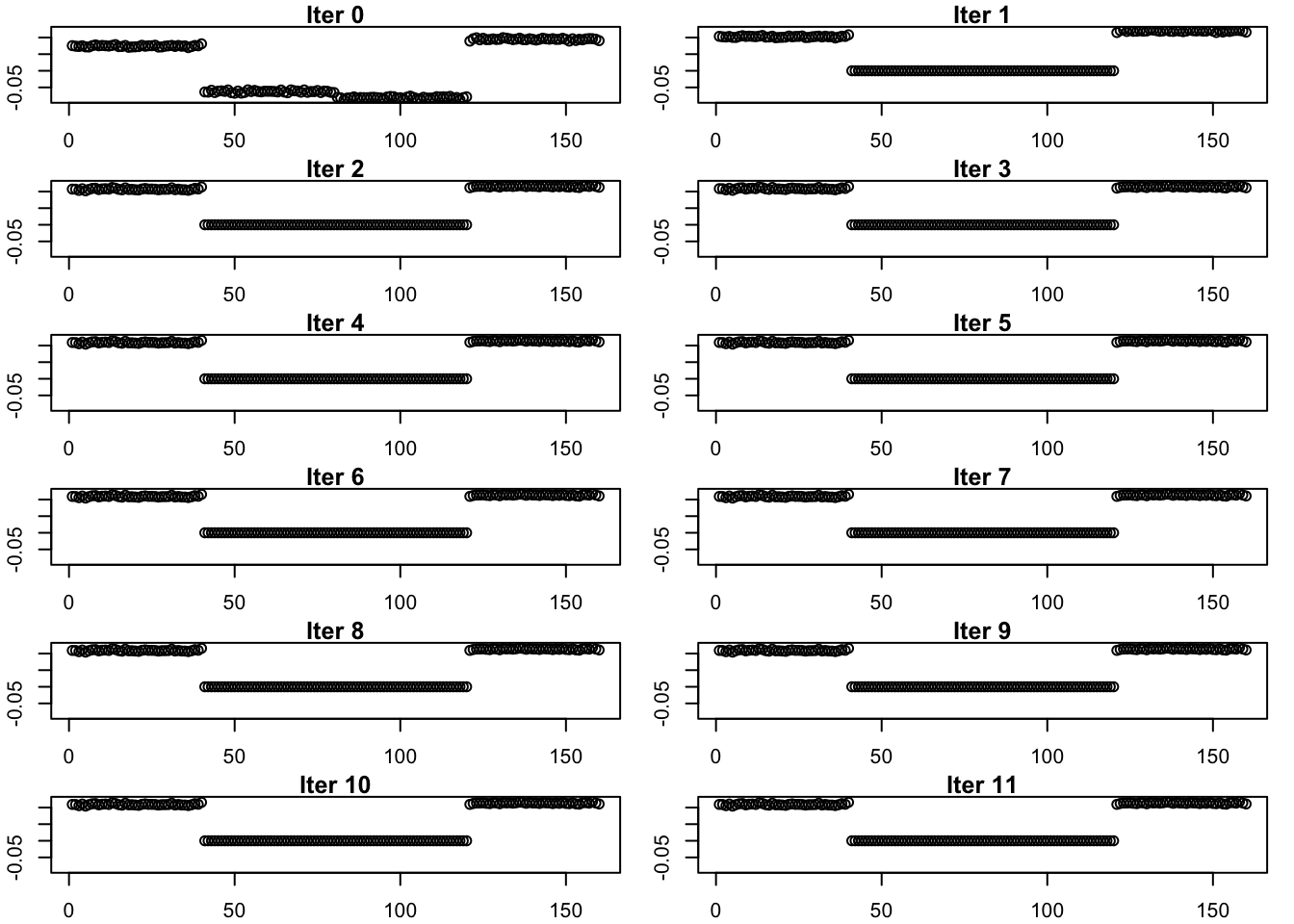
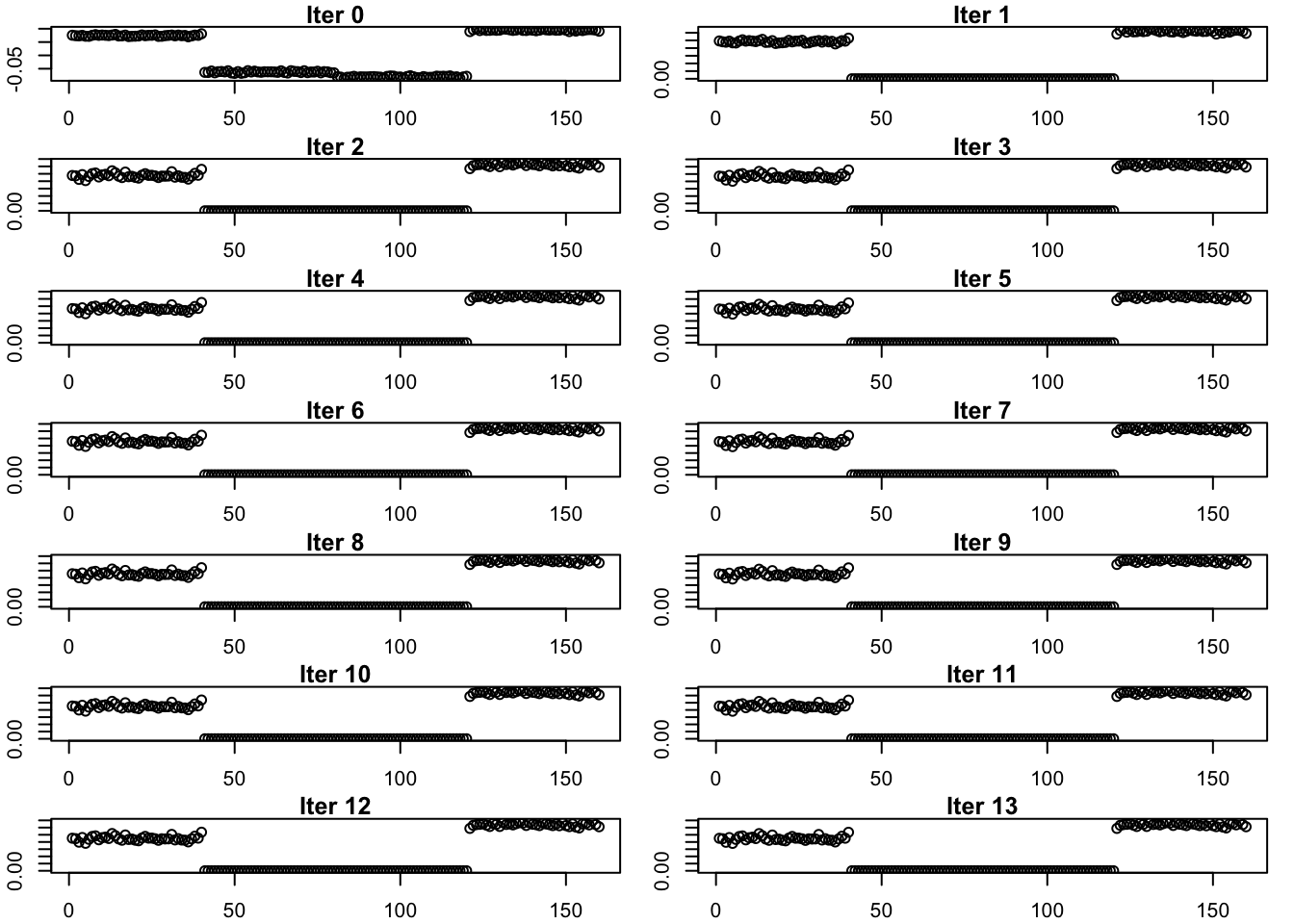
Progression of Estimate
R_exp <- sim_data$YYt - tcrossprod(symebcovmf_exp_init_fit$L_pm %*% diag(sqrt(symebcovmf_exp_init_fit$lambda), ncol = 3))
estimates_exp_list <- list(sym_ebcovmf_r1_init(R_exp)$v)
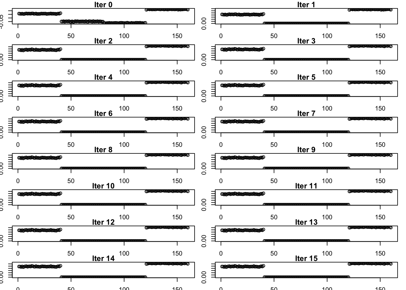
for (i in 1:13){
estimates_exp_list[[(i+1)]] <- sym_ebcovmf_r1_fit(sim_data$YYt, symebcovmf_exp_init_fit, ebnm_fn = ebnm::ebnm_point_exponential, maxiter = i, tol = 10^(-8))$L_pm[,4]
}par(mfrow = c(7,2), mar = c(2, 2, 1, 1) + 0.1)
for (i in 1:14){
plot(estimates_exp_list[[i]], main = paste('Iter', (i-1)), ylab = 'L')
}
par(mfrow = c(1,1))plot_heatmap(R_exp, colors_range = c('blue','gray96','red'), brks = seq(-max(abs(R_exp)), max(abs(R_exp)), length.out = 50))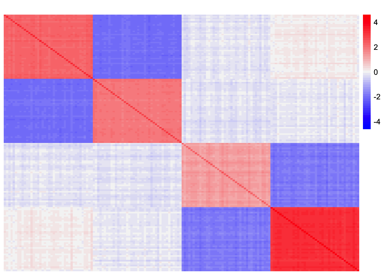
| Version | Author | Date |
|---|---|---|
| a7697e5 | Annie Xie | 2025-04-15 |
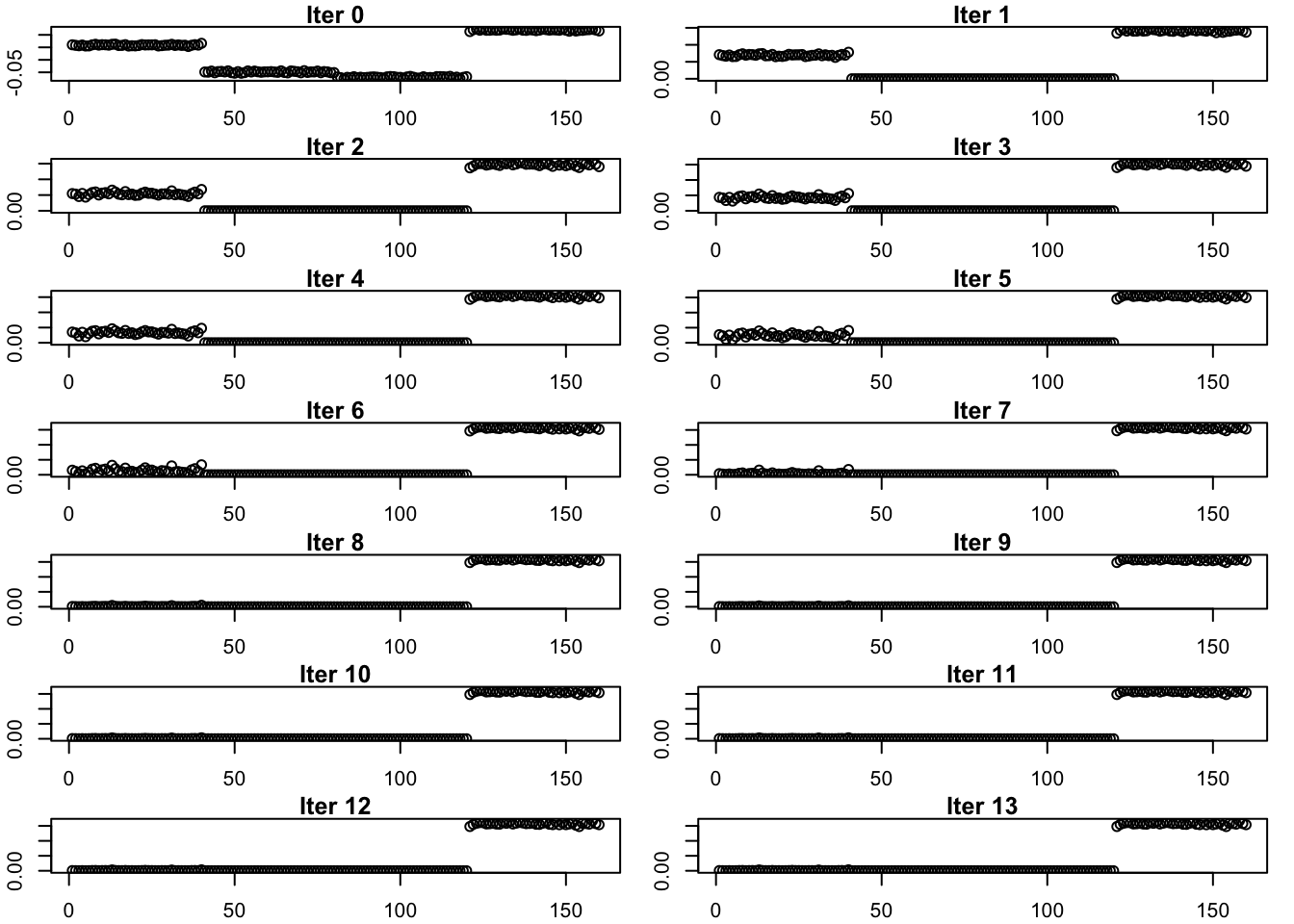
Generalized binary prior
symebcovmf_gb_fit <- sym_ebcovmf_r1_fit(sim_data$YYt, symebcovmf_gb_init_fit, ebnm_fn = ebnm::ebnm_generalized_binary, maxiter = 500, tol = 10^(-8))
symebcovmf_gb_fit <- refit_lambda(sim_data$YYt, symebcovmf_gb_fit)
Visualization of Estimate
plot(symebcovmf_gb_fit$L_pm[,4])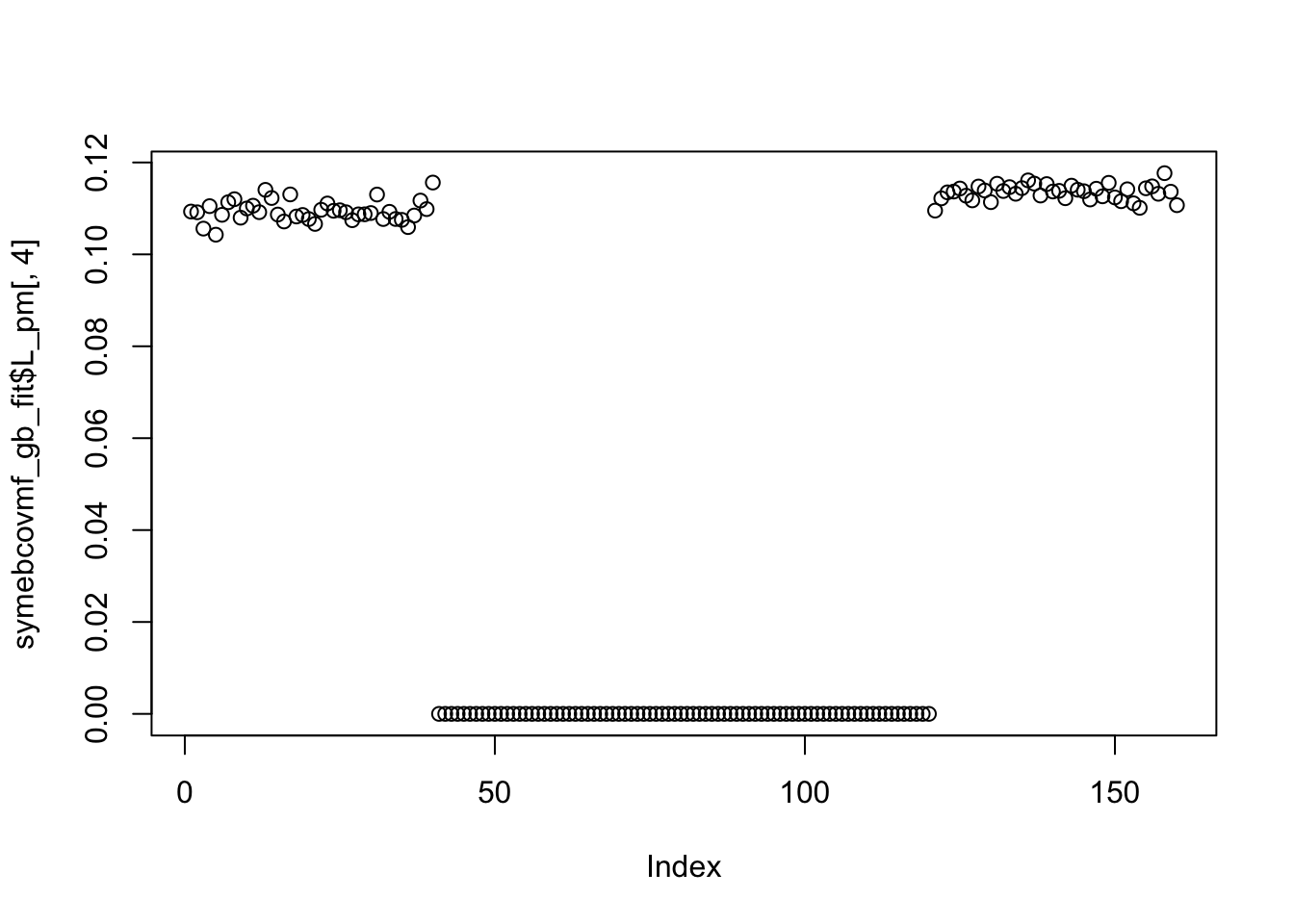
Visualization of ELBO
This is a plot of the progression of the ELBO:
idx <- which(symebcovmf_gb_fit$vec_elbo_full == 4)
plot(symebcovmf_gb_fit$vec_elbo_full[-c(1:idx)], type = 'b', xlab = 'Iter', ylab = 'ELBO') 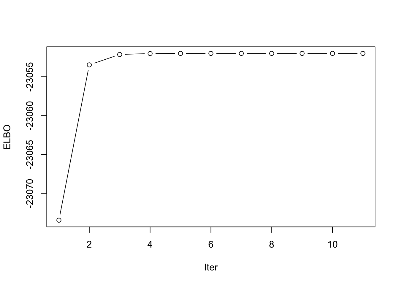
Progression of Estimate
R_gb <- sim_data$YYt - tcrossprod(symebcovmf_gb_init_fit$L_pm %*% diag(sqrt(symebcovmf_gb_init_fit$lambda), ncol = 3))
estimates_gb_list <- list(sym_ebcovmf_r1_init(R_gb)$v)
for (i in 1:11){
  estimates_gb_list[[(i+1)]] <- sym_ebcovmf_r1_fit(sim_data$YYt, symebcovmf_gb_init_fit, ebnm_fn = ebnm::ebnm_generalized_binary, maxiter = i, tol = 10^(-8))$L_pm[,4]
}
par(mfrow = c(6,2), mar = c(2, 2, 1, 1) + 0.1)
max_y <- max(sapply(estimates_gb_list, max))
min_y <- min(sapply(estimates_gb_list, min))
for (i in 1:12){
plot(estimates_gb_list[[i]], main = paste('Iter', (i-1)), ylab = 'L', ylim = c(min_y, max_y))
}
par(mfrow = c(1,1))plot_heatmap(R_gb, colors_range = c('blue','gray96','red'), brks = seq(-max(abs(R_gb)), max(abs(R_gb)), length.out = 50))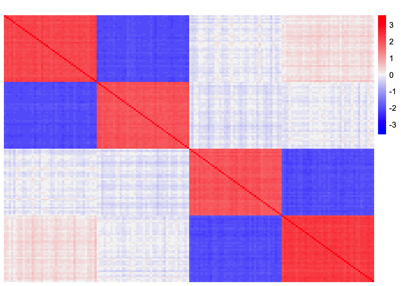
| Version | Author | Date |
|---|---|---|
| bbe7534 | Annie Xie | 2025-04-21 |
Observations
We can see that point-exponential prior is able to find a sparser solution in this setting. On the other hand, the generalized binary prior found a less sparse, binary solution. Something to try in the future: if I initialize the generalized-binary prior fit with the correct factor, will it recover something close to the correct factor? General question: how sensitive is the generalized binary prior to initialization? My guess is it would be pretty sensitive.
Mixing point-exponential and generalized binary
I want to try fitting the fourth factor with a point-exponential prior, but using the generalized-binary fit for the first three factors. I’m interested in this because I am interested in developing an procedure that uses the point-exponential prior as an initialization, and then refines the fit with a binary or generalized-binary prior.
Point-exponential prior
symebcovmf_exp_gb_fit <- sym_ebcovmf_r1_fit(sim_data$YYt, symebcovmf_gb_init_fit, ebnm_fn = ebnm::ebnm_point_exponential, maxiter = 500, tol = 10^(-8))
symebcovmf_exp_gb_fit <- refit_lambda(sim_data$YYt, symebcovmf_exp_gb_fit)
Visualization of Estimate
plot(symebcovmf_exp_gb_fit$L_pm[,4])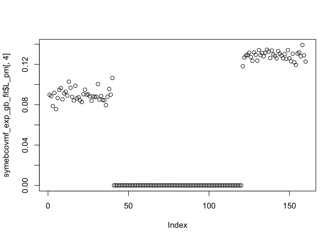
Visualization of ELBO
This is a plot of the progression of the ELBO:
idx <- which(symebcovmf_exp_gb_fit$vec_elbo_full == 4)
plot(symebcovmf_exp_gb_fit$vec_elbo_full[-c(1:idx)], type = 'b', xlab = 'Iter', ylab = 'ELBO') 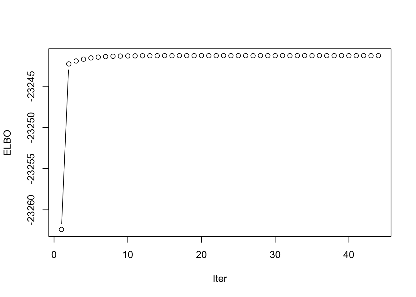
| Version | Author | Date |
|---|---|---|
| bbe7534 | Annie Xie | 2025-04-21 |
Progression of Estimate
#R_gb <- sim_data$YYt - tcrossprod(symebcovmf_gb_init_fit$L_pm %*% diag(sqrt(symebcovmf_gb_init_fit$lambda), ncol = 3))
estimates_exp_gb_list <- list(sym_ebcovmf_r1_init(R_gb)$v)
for (i in 1:13){
  estimates_exp_gb_list[[(i+1)]] <- sym_ebcovmf_r1_fit(sim_data$YYt, symebcovmf_gb_init_fit, ebnm_fn = ebnm::ebnm_point_exponential, maxiter = i, tol = 10^(-8))$L_pm[,4]
}
par(mfrow = c(7,2), mar = c(2, 2, 1, 1) + 0.1)
for (i in 1:14){
plot(estimates_exp_gb_list[[i]], main = paste('Iter', (i-1)), ylab = 'L')
}
par(mfrow = c(1,1))Observations
Using the point-exponential prior to fit the fourth factor from the generalized-binary fit, we see that the fourth factor does not capture a singular population effect. Instead, it captures two populations. This suggests that the point-exponential prior alone may not be enough to get a sparse solution. Looking at the residual matrices and the eigenvalues, it looks like there is better separation between the first and second eigenvalue of the residual matrix from the point-exponential fit compared to that of the generalized-binary fit. Therefore, that may make it easier for the method to find only one population effect as a factor vs. grouping together effects.
Generalized binary prior
symebcovmf_gb_exp_fit <- sym_ebcovmf_r1_fit(sim_data$YYt, symebcovmf_exp_init_fit, ebnm_fn = ebnm::ebnm_generalized_binary, maxiter = 500, tol = 10^(-8))
symebcovmf_gb_exp_fit <- refit_lambda(sim_data$YYt, symebcovmf_gb_exp_fit)
Visualization of Estimate
plot(symebcovmf_gb_exp_fit$L_pm[,4])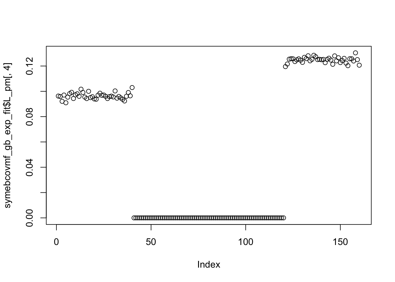
Visualization of ELBO
This is a plot of the progression of the ELBO:
idx <- which(symebcovmf_gb_exp_fit$vec_elbo_full == 4)
plot(symebcovmf_gb_exp_fit$vec_elbo_full[-c(1:idx)], type = 'b', xlab = 'Iter', ylab = 'ELBO') 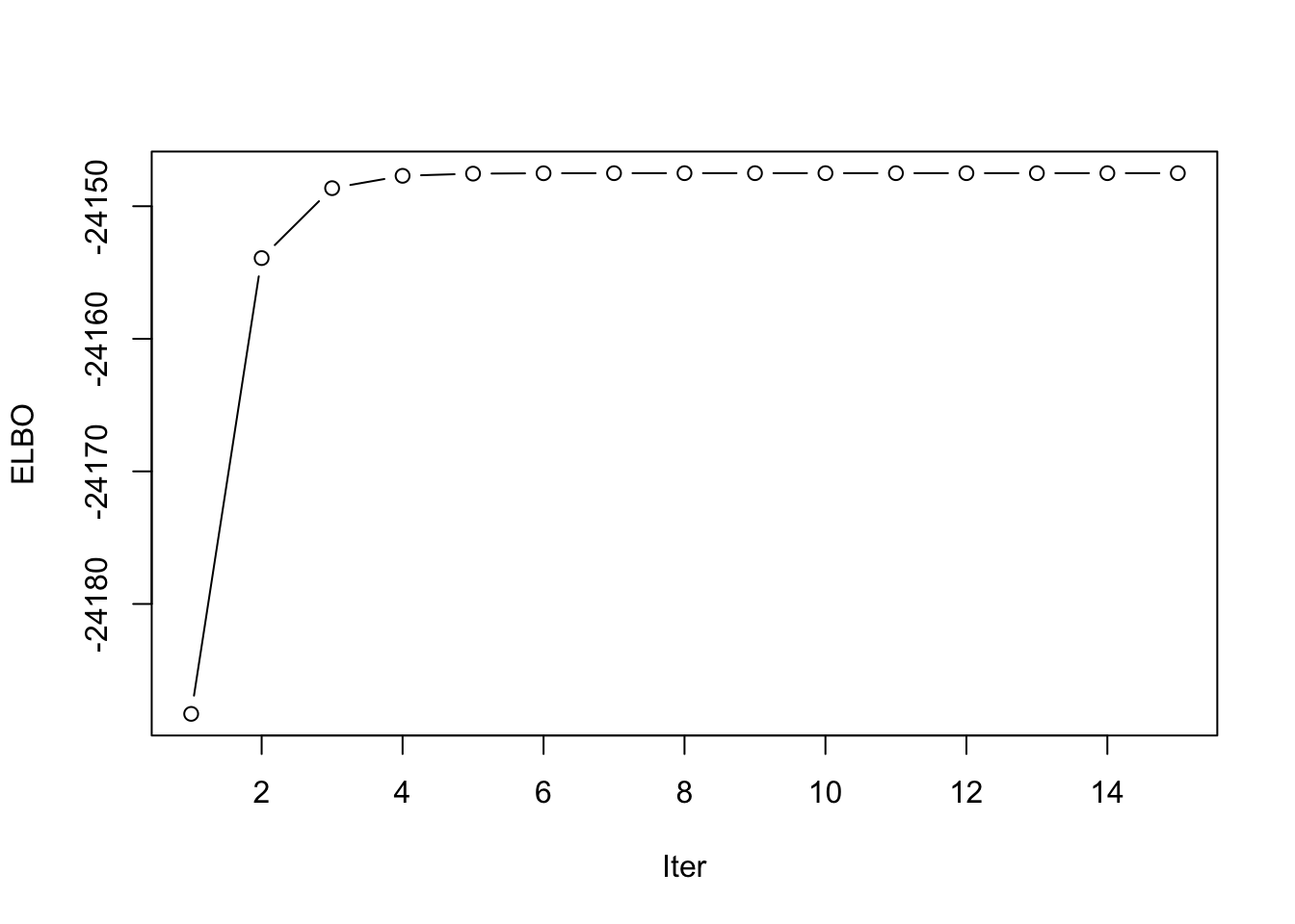
| Version | Author | Date |
|---|---|---|
| bbe7534 | Annie Xie | 2025-04-21 |
Progression of Estimate
#R_gb <- sim_data$YYt - tcrossprod(symebcovmf_gb_init_fit$L_pm %*% diag(sqrt(symebcovmf_gb_init_fit$lambda), ncol = 3))
estimates_gb_exp_list <- list(sym_ebcovmf_r1_init(R_exp)$v)
for (i in 1:15){
  estimates_gb_exp_list[[(i+1)]] <- sym_ebcovmf_r1_fit(sim_data$YYt, symebcovmf_exp_init_fit, ebnm_fn = ebnm::ebnm_generalized_binary, maxiter = i, tol = 10^(-8))$L_pm[,4]
}
par(mfrow = c(8,2), mar = c(1.5, 1.5, 1, 1) + 0.1)
for (i in 1:16){
plot(estimates_gb_exp_list[[i]], main = paste('Iter', (i-1)), ylab = 'L')
}
par(mfrow = c(1,1))Observations
Using generalized binary for the fourth factor on the point-exponential fit yields an estimate that does not look like a population effect. Similar to other estimates, the factor captures the effect of two populations. Comparing generalized binary and point-exponential for fitting the fourth factor on the point-exponential fit, we see that the point-exponential prior is better at yielding sparse estimates than generalized-binary. The estimate that generalized binary finds is in line with what the prior encourages. Note that since we are using the generalized binary prior, there is nothing constraining the prior to be exactly binary.
sessionInfo()R version 4.3.2 (2023-10-31)
Platform: aarch64-apple-darwin20 (64-bit)
Running under: macOS Sonoma 14.4.1
Matrix products: default
BLAS: /Library/Frameworks/R.framework/Versions/4.3-arm64/Resources/lib/libRblas.0.dylib
LAPACK: /Library/Frameworks/R.framework/Versions/4.3-arm64/Resources/lib/libRlapack.dylib; LAPACK version 3.11.0
locale:
[1] en_US.UTF-8/en_US.UTF-8/en_US.UTF-8/C/en_US.UTF-8/en_US.UTF-8
time zone: America/Chicago
tzcode source: internal
attached base packages:
[1] stats graphics grDevices utils datasets methods base
other attached packages:
[1] ggplot2_3.5.1 pheatmap_1.0.12 ebnm_1.1-34 workflowr_1.7.1
loaded via a namespace (and not attached):
[1] gtable_0.3.5 xfun_0.48 bslib_0.8.0 processx_3.8.4
[5] lattice_0.22-6 callr_3.7.6 vctrs_0.6.5 tools_4.3.2
[9] ps_1.7.7 generics_0.1.3 tibble_3.2.1 fansi_1.0.6
[13] highr_0.11 pkgconfig_2.0.3 Matrix_1.6-5 SQUAREM_2021.1
[17] RColorBrewer_1.1-3 lifecycle_1.0.4 truncnorm_1.0-9 farver_2.1.2
[21] compiler_4.3.2 stringr_1.5.1 git2r_0.33.0 munsell_0.5.1
[25] getPass_0.2-4 httpuv_1.6.15 htmltools_0.5.8.1 sass_0.4.9
[29] yaml_2.3.10 later_1.3.2 pillar_1.9.0 jquerylib_0.1.4
[33] whisker_0.4.1 cachem_1.1.0 trust_0.1-8 RSpectra_0.16-2
[37] tidyselect_1.2.1 digest_0.6.37 stringi_1.8.4 dplyr_1.1.4
[41] ashr_2.2-66 labeling_0.4.3 splines_4.3.2 rprojroot_2.0.4
[45] fastmap_1.2.0 grid_4.3.2 colorspace_2.1-1 cli_3.6.3
[49] invgamma_1.1 magrittr_2.0.3 utf8_1.2.4 withr_3.0.1
[53] scales_1.3.0 promises_1.3.0 horseshoe_0.2.0 rmarkdown_2.28
[57] httr_1.4.7 deconvolveR_1.2-1 evaluate_1.0.0 knitr_1.48
[61] irlba_2.3.5.1 rlang_1.1.4 Rcpp_1.0.13 mixsqp_0.3-54
[65] glue_1.8.0 rstudioapi_0.16.0 jsonlite_1.8.9 R6_2.5.1
[69] fs_1.6.4