Last updated: 2025-04-21

Checks: 7 0

Knit directory: symmetric_covariance_decomposition/

This reproducible R Markdown analysis was created with workflowr (version 1.7.1). The Checks tab describes the reproducibility checks that were applied when the results were created. The Past versions tab lists the development history.

R Markdown file: up-to-date

Great! Since the R Markdown file has been committed to the Git repository, you know the exact version of the code that produced these results.

Environment: empty

Great job! The global environment was empty. Objects defined in the global environment can affect the analysis in your R Markdown file in unknown ways. For reproduciblity it’s best to always run the code in an empty environment.

Seed: set.seed(20250408)

The command set.seed(20250408) was run prior to running the code in the R Markdown file. Setting a seed ensures that any results that rely on randomness, e.g. subsampling or permutations, are reproducible.

Session information: recorded

Great job! Recording the operating system, R version, and package versions is critical for reproducibility.

Cache: none

Nice! There were no cached chunks for this analysis, so you can be confident that you successfully produced the results during this run.

File paths: relative

Great job! Using relative paths to the files within your workflowr project makes it easier to run your code on other machines.

Repository version: b16d9c5

Great! You are using Git for version control. Tracking code development and connecting the code version to the results is critical for reproducibility.

The results in this page were generated with repository version b16d9c5. See the Past versions tab to see a history of the changes made to the R Markdown and HTML files.

Note that you need to be careful to ensure that all relevant files for the analysis have been committed to Git prior to generating the results (you can use wflow_publish or wflow_git_commit). workflowr only checks the R Markdown file, but you know if there are other scripts or data files that it depends on. Below is the status of the Git repository when the results were generated:


Ignored files:
    Ignored:    .DS_Store
    Ignored:    .Rhistory

Note that any generated files, e.g. HTML, png, CSS, etc., are not included in this status report because it is ok for generated content to have uncommitted changes.

These are the previous versions of the repository in which changes were made to the R Markdown (analysis/symebcovmf_tree.Rmd) and HTML (docs/symebcovmf_tree.html) files. If you’ve configured a remote Git repository (see ?wflow_git_remote), click on the hyperlinks in the table below to view the files as they were in that past version.

File	Version	Author	Date	Message
Rmd	b16d9c5	Annie Xie	2025-04-21	Update symebcovmf tree analysis
html	e0e8add	Annie Xie	2025-04-08	Build site.
Rmd	1be0238	Annie Xie	2025-04-08	Add symebcovmf analysis files

Introduction

In this example, we test out symEBcovMF on tree-structured data.

Example

library(ebnm)
library(pheatmap)
library(ggplot2)

source('code/symebcovmf_functions.R')
source('code/visualization_functions.R')

Data Generation

sim_4pops <- function(args) {
  set.seed(args$seed)
  
  n <- sum(args$pop_sizes)
  p <- args$n_genes
  
  FF <- matrix(rnorm(7 * p, sd = rep(args$branch_sds, each = p)), ncol = 7)
  # if (args$constrain_F) {
  #   FF_svd <- svd(FF)
  #   FF <- FF_svd$u
  #   FF <- t(t(FF) * branch_sds * sqrt(p))
  # }
  
  LL <- matrix(0, nrow = n, ncol = 7)
  LL[, 1] <- 1
  LL[, 2] <- rep(c(1, 1, 0, 0), times = args$pop_sizes)
  LL[, 3] <- rep(c(0, 0, 1, 1), times = args$pop_sizes)
  LL[, 4] <- rep(c(1, 0, 0, 0), times = args$pop_sizes)
  LL[, 5] <- rep(c(0, 1, 0, 0), times = args$pop_sizes)
  LL[, 6] <- rep(c(0, 0, 1, 0), times = args$pop_sizes)
  LL[, 7] <- rep(c(0, 0, 0, 1), times = args$pop_sizes)
  
  E <- matrix(rnorm(n * p, sd = args$indiv_sd), nrow = n)
  Y <- LL %*% t(FF) + E
  YYt <- (1/p)*tcrossprod(Y)
  return(list(Y = Y, YYt = YYt, LL = LL, FF = FF, K = ncol(LL)))
}

sim_args = list(pop_sizes = rep(40, 4), n_genes = 1000, branch_sds = rep(2,7), indiv_sd = 1, seed = 1)
sim_data <- sim_4pops(sim_args)

This is a heatmap of the scaled Gram matrix:

plot_heatmap(sim_data$YYt, colors_range = c('blue','gray96','red'), brks = seq(-max(abs(sim_data$YYt)), max(abs(sim_data$YYt)), length.out = 50))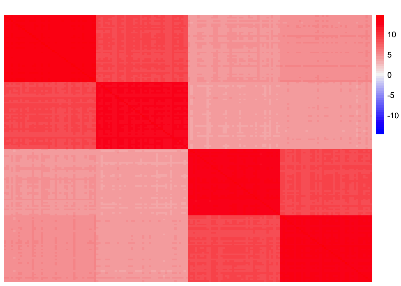

Version	Author	Date
e0e8add	Annie Xie	2025-04-08

This is a scatter plot of the true loadings matrix:

pop_vec <- c(rep('A', 40), rep('B', 40), rep('C', 40), rep('D', 40))
plot_loadings(sim_data$LL, pop_vec)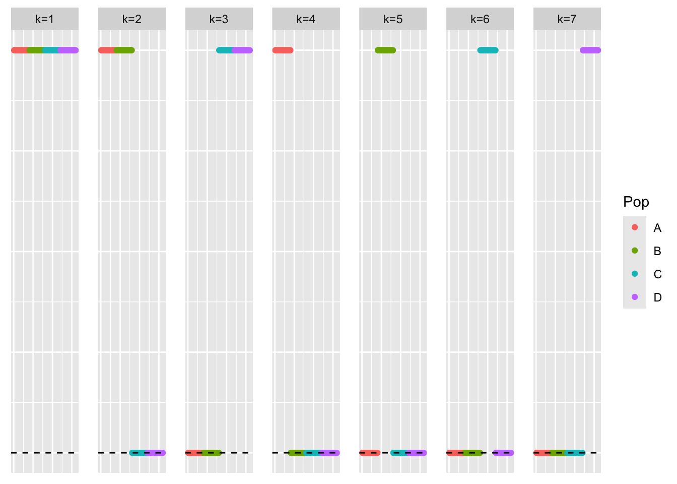

Version	Author	Date
e0e8add	Annie Xie	2025-04-08

symEBcovMF

symebcovmf_tree_fit <- sym_ebcovmf_fit(S = sim_data$YYt, ebnm_fn = ebnm_point_exponential, K = 7, maxiter = 100, rank_one_tol = 10^(-8), tol = 10^(-8))

[1] "Warning: scaling factor is zero"
[1] "Adding factor 4 does not improve the objective function"

Progression of ELBO

symebcovmf_tree_full_elbo_vec <- symebcovmf_tree_fit$vec_elbo_full[!(symebcovmf_tree_fit$vec_elbo_full %in% c(1:length(symebcovmf_tree_fit$vec_elbo_K)))]
ggplot() + geom_line(data = NULL, aes(x = 1:length(symebcovmf_tree_full_elbo_vec), y = symebcovmf_tree_full_elbo_vec)) + xlab('Iter') + ylab('ELBO')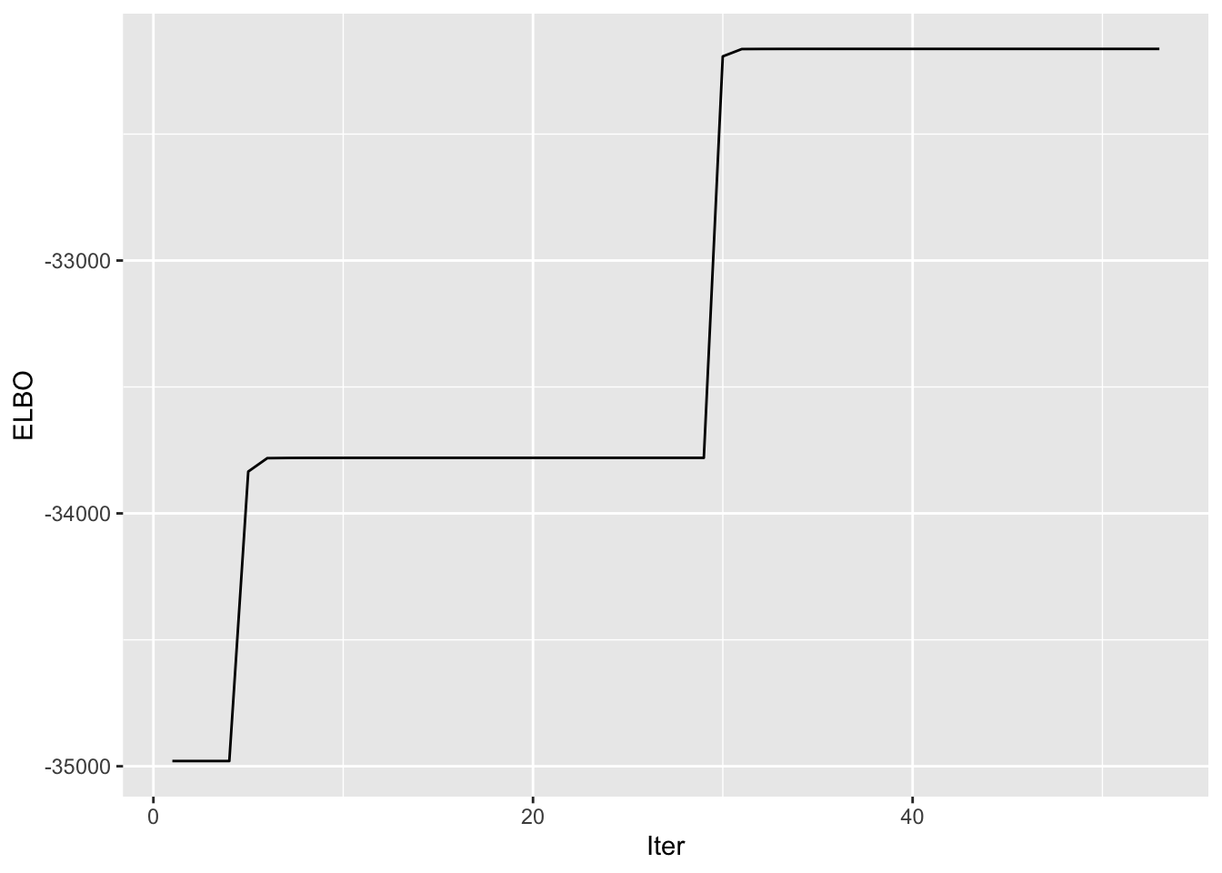

Version	Author	Date
e0e8add	Annie Xie	2025-04-08

Visualization of Estimate

This is a scatter plot of \(\hat{L}\), the estimate from symEBcovMF:

bal_pops <- c(rep('A', 40), rep('B', 40), rep('C', 40), rep('D', 40))
plot_loadings(symebcovmf_tree_fit$L_pm %*% diag(sqrt(symebcovmf_tree_fit$lambda)), bal_pops)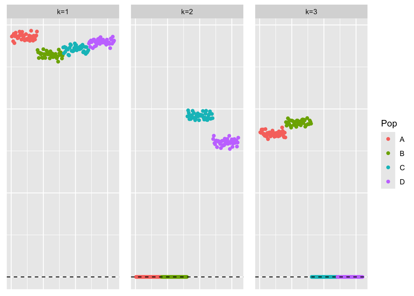

Version	Author	Date
e0e8add	Annie Xie	2025-04-08

This is the objective function value attained:

symebcovmf_tree_fit$elbo

[1] -32163.04

Visualization of Fit

This is a heatmap of \(\hat{L}\hat{\Lambda}\hat{L}'\):

symebcovmf_tree_fitted_vals <- tcrossprod(symebcovmf_tree_fit$L_pm %*% diag(sqrt(symebcovmf_tree_fit$lambda)))
plot_heatmap(symebcovmf_tree_fitted_vals, brks = seq(0, max(symebcovmf_tree_fitted_vals), length.out = 50))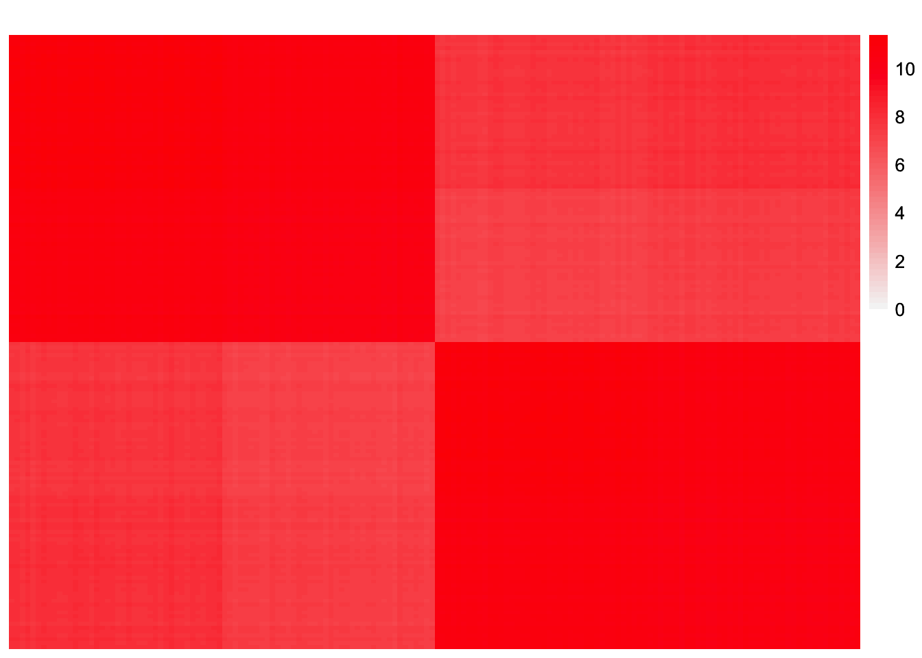

Version	Author	Date
e0e8add	Annie Xie	2025-04-08

This is a scatter plot of fitted values vs. observed values for the off-diagonal entries:

diag_idx <- seq(1, prod(dim(sim_data$YYt)), length.out = ncol(sim_data$YYt))
off_diag_idx <- setdiff(c(1:prod(dim(sim_data$YYt))), diag_idx) 

ggplot(data = NULL, aes(x = c(sim_data$YYt)[off_diag_idx], y = c(symebcovmf_tree_fitted_vals)[off_diag_idx])) + geom_point() + ylim(-1, 15) + xlim(-1,15) + xlab('Observed Values') + ylab('Fitted Values') + geom_abline(slope = 1, intercept = 0, color = 'red')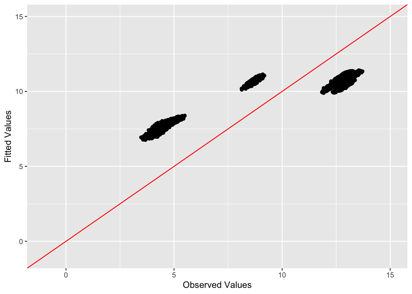

Version	Author	Date
e0e8add	Annie Xie	2025-04-08

Visualization of Residual Matrix

symebcovmf_tree_resid <- sim_data$YYt - symebcovmf_tree_fitted_vals
plot_heatmap(symebcovmf_tree_resid, colors_range = c('blue','gray96','red'), brks = seq(-max(abs(symebcovmf_tree_resid)), max(abs(symebcovmf_tree_resid)), length.out = 50))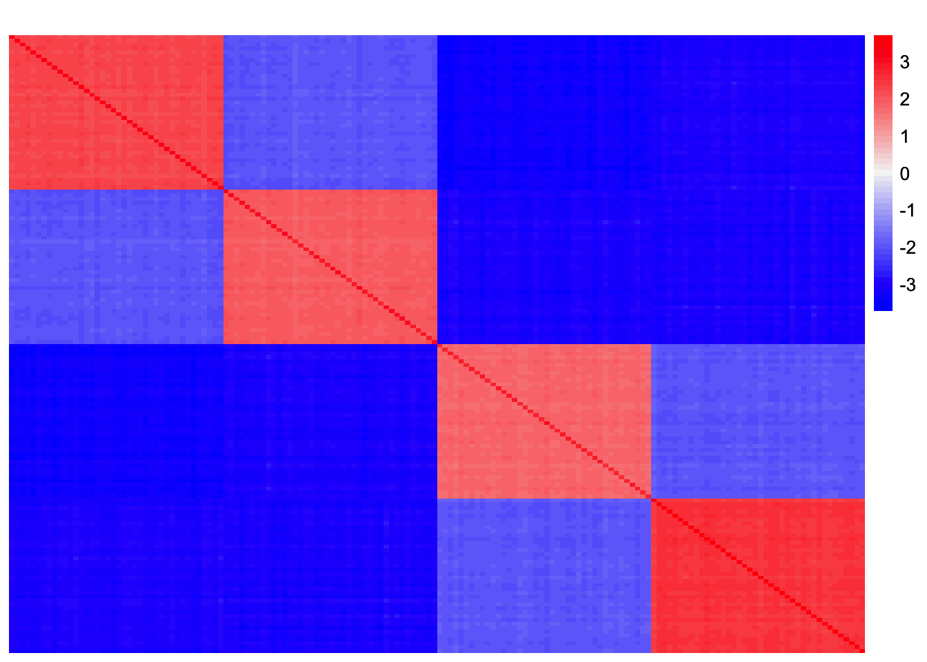

Version	Author	Date
e0e8add	Annie Xie	2025-04-08

Observations

symEBcovMF struggles in the tree setting. Similar to EBMFcov, symEBcovMF only recovers three factors, one intercept factor and two subtype specific factors. I suspect symEBcovMF has similar issues to EBMFcov where the residual matrix has large chunks of negative entries that cause it to not add anymore factors.

symEBcovMF with refit step

symebcovmf_tree_refit_fit <- sym_ebcovmf_fit(S = sim_data$YYt, ebnm_fn = ebnm_point_exponential, K = 7, maxiter = 100, rank_one_tol = 10^(-8), tol = 10^(-8), refit_lam = TRUE)

Progression of ELBO

symebcovmf_tree_refit_full_elbo_vec <- symebcovmf_tree_refit_fit$vec_elbo_full[!(symebcovmf_tree_refit_fit$vec_elbo_full %in% c(1:length(symebcovmf_tree_refit_fit$vec_elbo_K)))]
ggplot() + geom_line(data = NULL, aes(x = 1:length(symebcovmf_tree_refit_full_elbo_vec), y = symebcovmf_tree_refit_full_elbo_vec)) + xlab('Iter') + ylab('ELBO')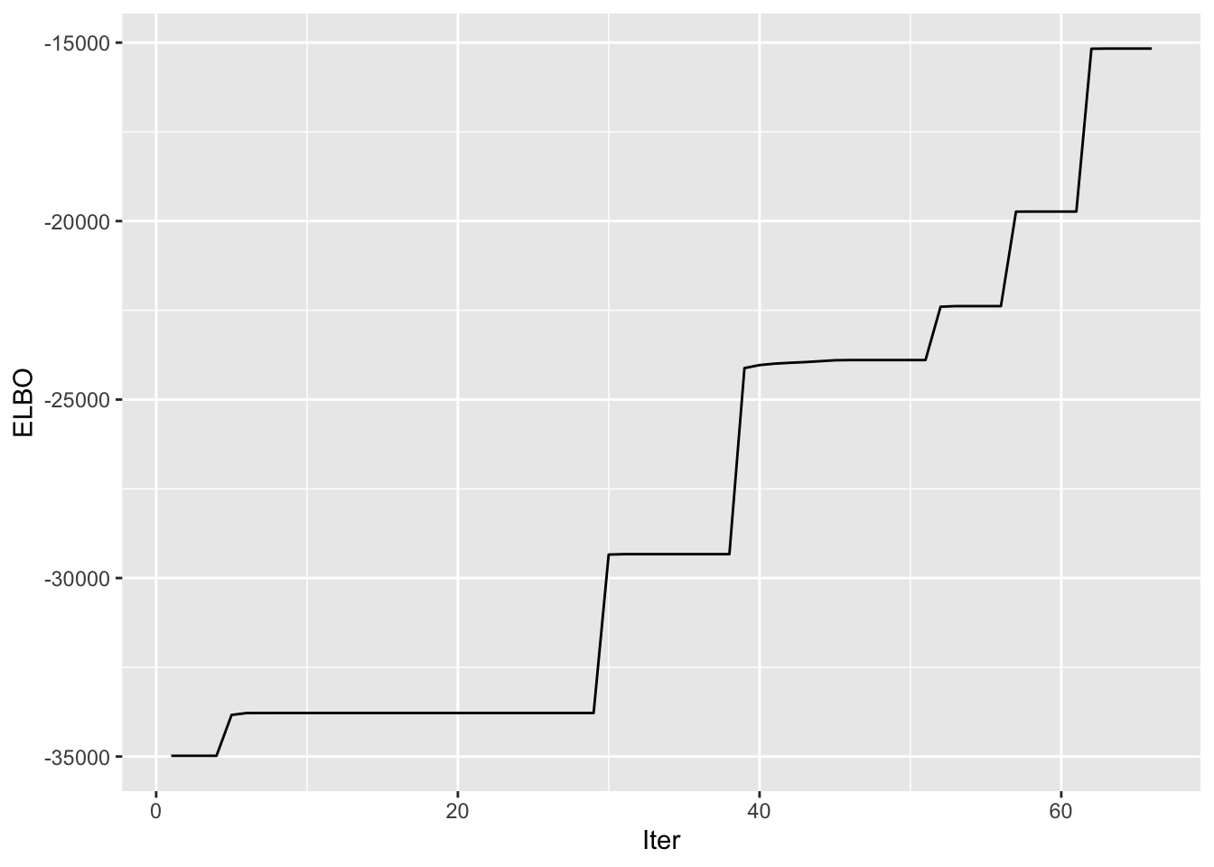

Version	Author	Date
e0e8add	Annie Xie	2025-04-08

A note: I don’t think I save the ELBO value after the refitting step in vec_elbo_full. But the refitting does change this vector since it changes the residual matrix that is used when you add a new vector.

Visualization of Estimate

This is a scatter plot of \(\hat{L}_{refit}\), the estimate from symEBcovMF:

bal_pops <- c(rep('A', 40), rep('B', 40), rep('C', 40), rep('D', 40))
plot_loadings(symebcovmf_tree_refit_fit$L_pm %*% diag(sqrt(symebcovmf_tree_refit_fit$lambda)), bal_pops)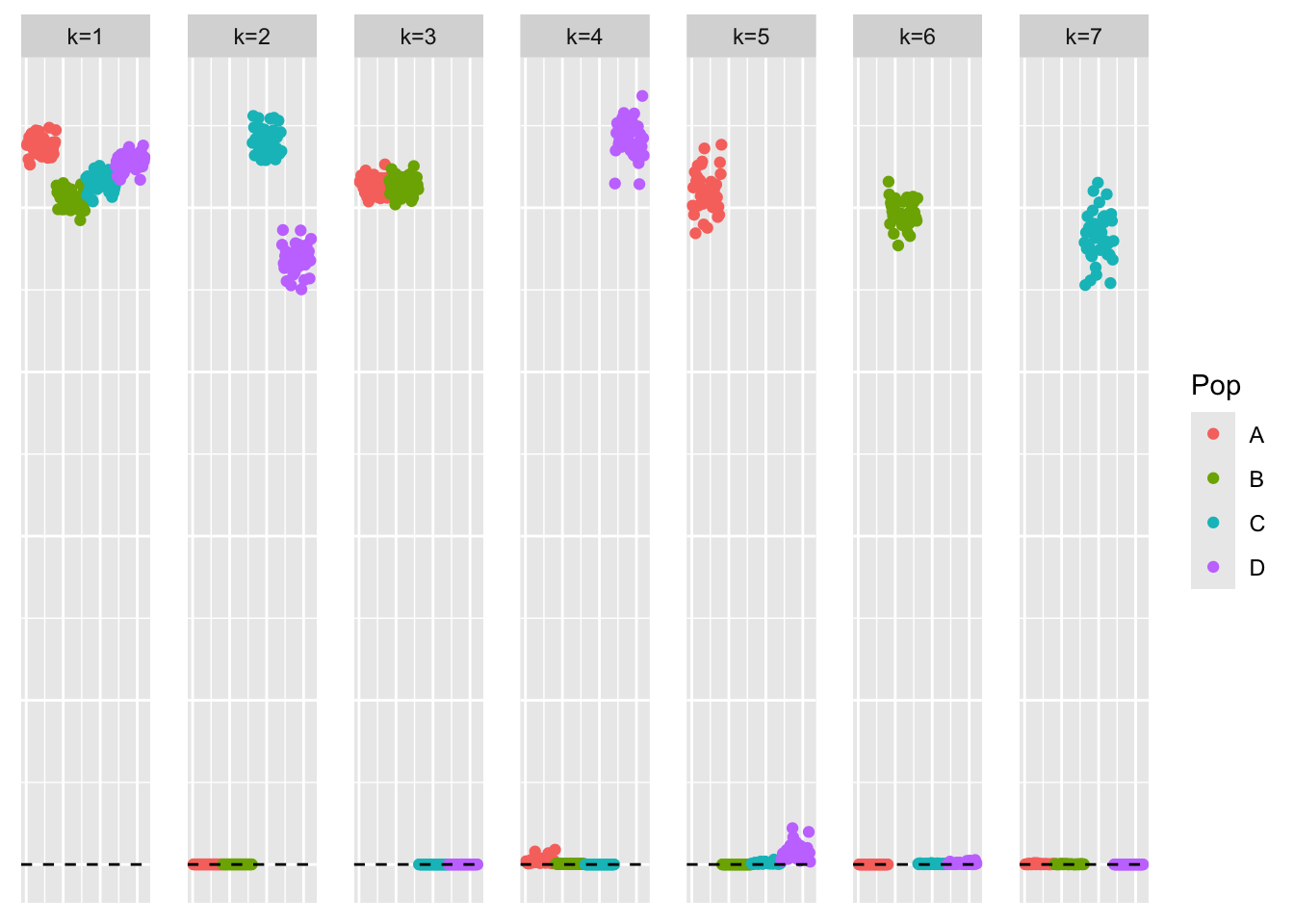

Version	Author	Date
e0e8add	Annie Xie	2025-04-08

This is the objective function value attained:

symebcovmf_tree_refit_fit$elbo

[1] -11576.24

Visualization of Fit

This is a heatmap of \(\hat{L}_{refit}\hat{\Lambda}_{refit}\hat{L}_{refit}'\):

symebcovmf_tree_refit_fitted_vals <- tcrossprod(symebcovmf_tree_refit_fit$L_pm %*% diag(sqrt(symebcovmf_tree_refit_fit$lambda)))
plot_heatmap(symebcovmf_tree_refit_fitted_vals, brks = seq(0, max(symebcovmf_tree_refit_fitted_vals), length.out = 50))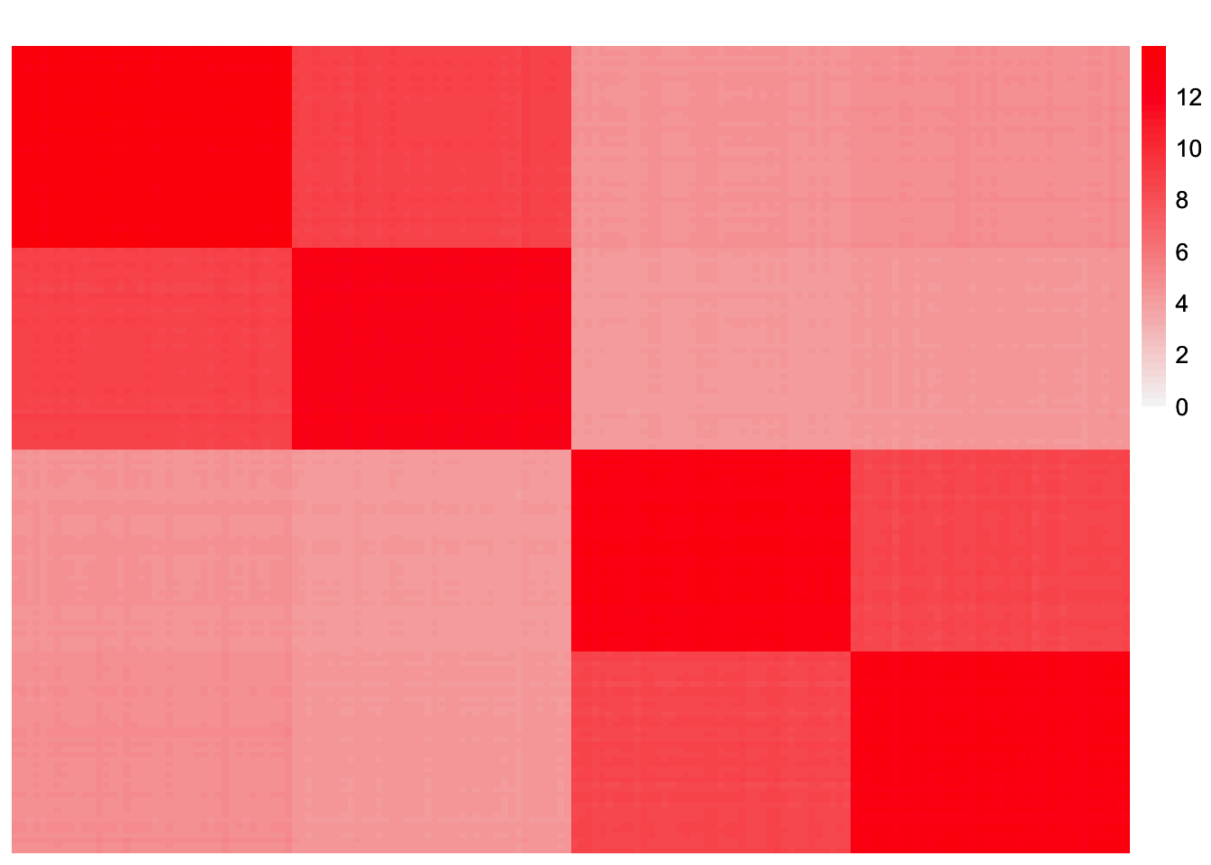

Version	Author	Date
e0e8add	Annie Xie	2025-04-08

This is a scatter plot of fitted values vs. observed values for the off-diagonal entries:

diag_idx <- seq(1, prod(dim(sim_data$YYt)), length.out = ncol(sim_data$YYt))
off_diag_idx <- setdiff(c(1:prod(dim(sim_data$YYt))), diag_idx) 

ggplot(data = NULL, aes(x = c(sim_data$YYt)[off_diag_idx], y = c(symebcovmf_tree_refit_fitted_vals)[off_diag_idx])) + geom_point() + ylim(-1, 15) + xlim(-1,15) + xlab('Observed Values') + ylab('Fitted Values') + geom_abline(slope = 1, intercept = 0, color = 'red')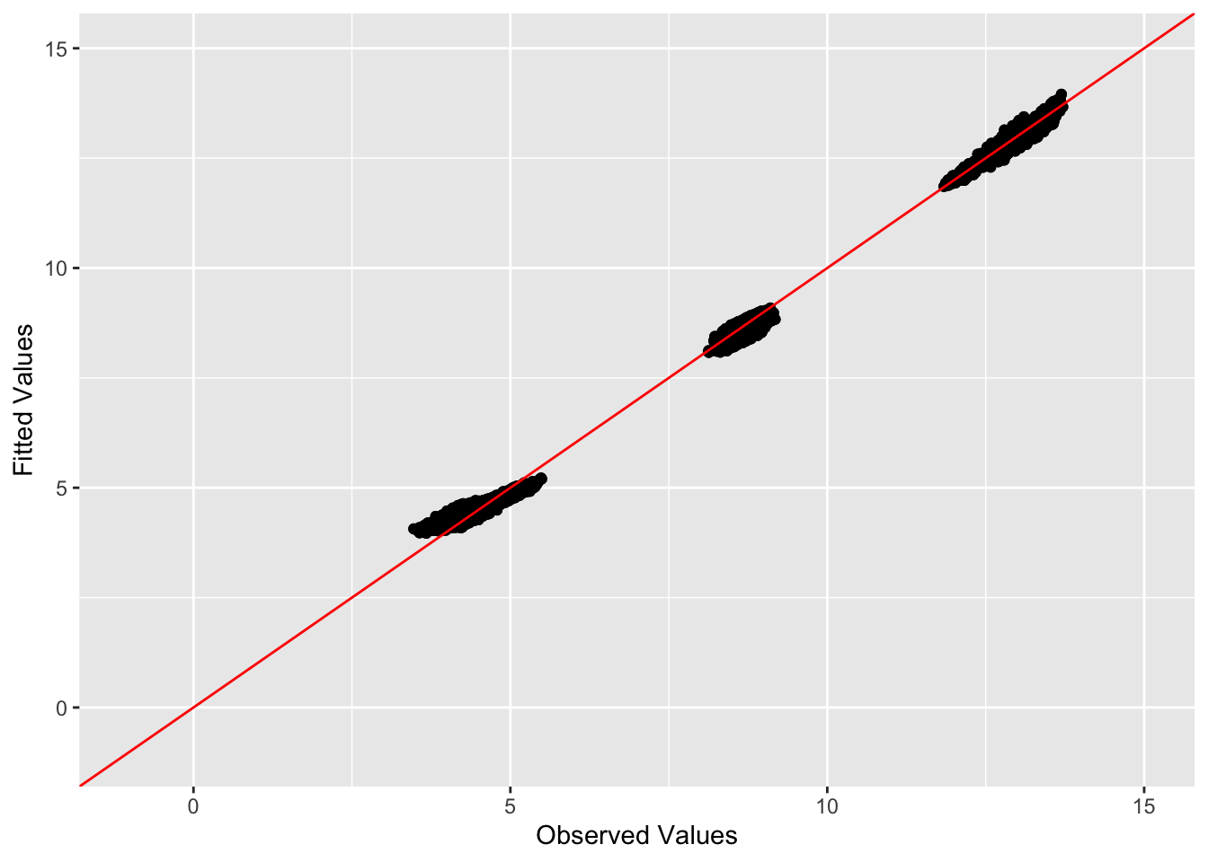

Version	Author	Date
e0e8add	Annie Xie	2025-04-08

Visualization of Residual Matrix

For comparison, I also plot a heatmap of \(S - \sum_{k=1}^{3} \hat{\lambda}_k \hat{\ell}_k \hat{\ell}_k\) where \(\hat{\lambda}_k\) and \(\hat{\ell}_k\) are estimates from symEBcovMF with the refitting step (note: in this visualization, we are using the estimate fit with 7 factors):

symebcovmf_tree_refit_resid <- sim_data$YYt - tcrossprod(symebcovmf_tree_refit_fit$L_pm[,c(1:3)] %*% diag(sqrt(symebcovmf_tree_refit_fit$lambda[1:3])))
plot_heatmap(symebcovmf_tree_refit_resid, colors_range = c('blue','gray96','red'), brks = seq(-max(abs(symebcovmf_tree_refit_resid)), max(abs(symebcovmf_tree_refit_resid)), length.out = 50))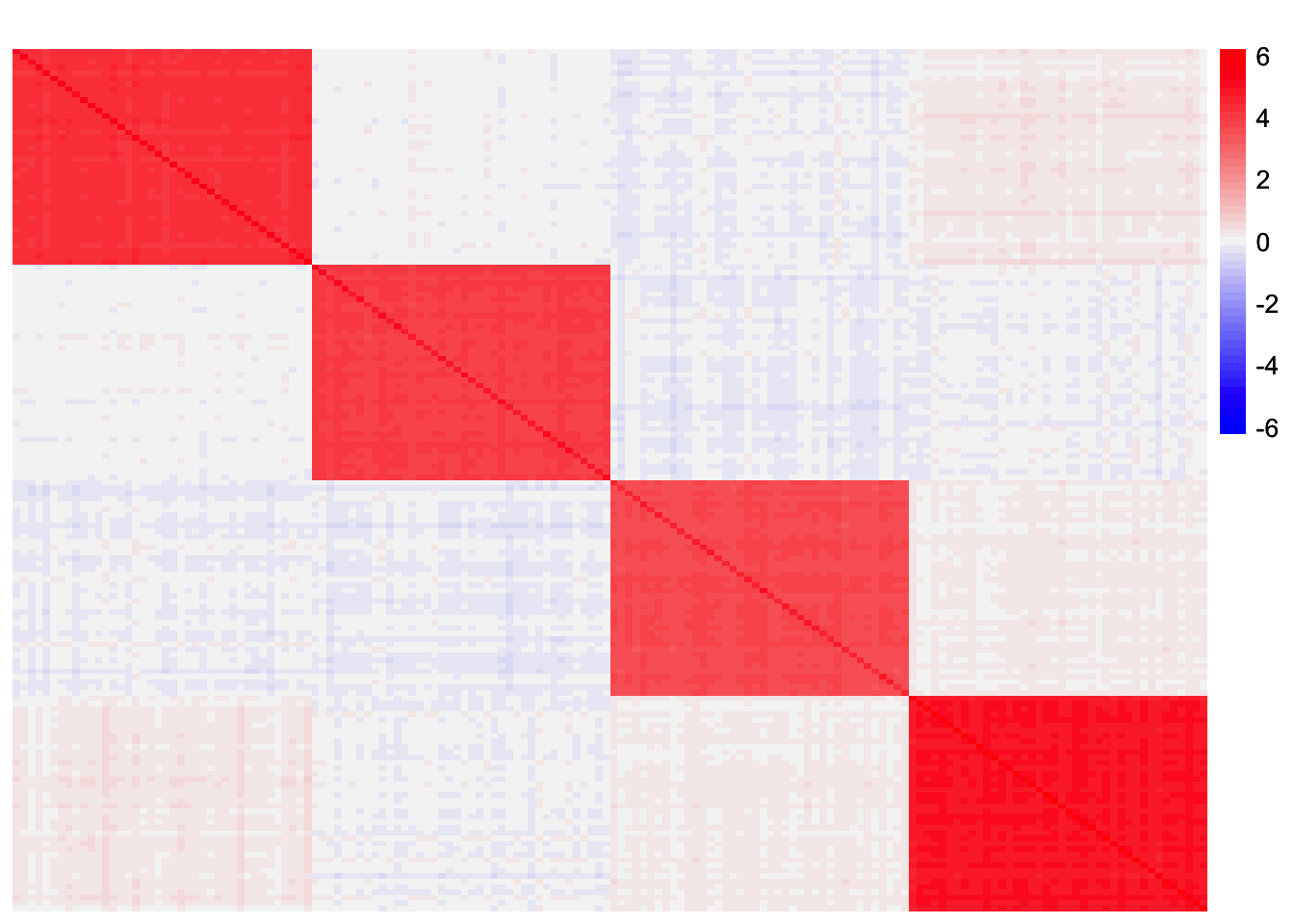

Version	Author	Date
e0e8add	Annie Xie	2025-04-08

Here, I plot a heatmap of \(S - \sum_{k=1}^{3} \hat{\lambda}_k \hat{\ell}_k \hat{\ell}_k\) where \(\hat{\lambda}_k\) and \(\hat{\ell}_k\) are estimates from symEBcovMF with the refitting step and Kmax = 3:

symebcovmf_tree_refit_k3_fit <- sym_ebcovmf_fit(S = sim_data$YYt, ebnm_fn = ebnm_point_exponential, K = 3, maxiter = 100, rank_one_tol = 10^(-8), tol = 10^(-8), refit_lam = TRUE)

symebcovmf_tree_refit_k3_resid <- sim_data$YYt - tcrossprod(symebcovmf_tree_refit_k3_fit$L_pm %*% diag(sqrt(symebcovmf_tree_refit_k3_fit$lambda)))
plot_heatmap(symebcovmf_tree_refit_k3_resid, colors_range = c('blue','gray96','red'), brks = seq(-max(abs(symebcovmf_tree_refit_k3_resid)), max(abs(symebcovmf_tree_refit_k3_resid)), length.out = 50))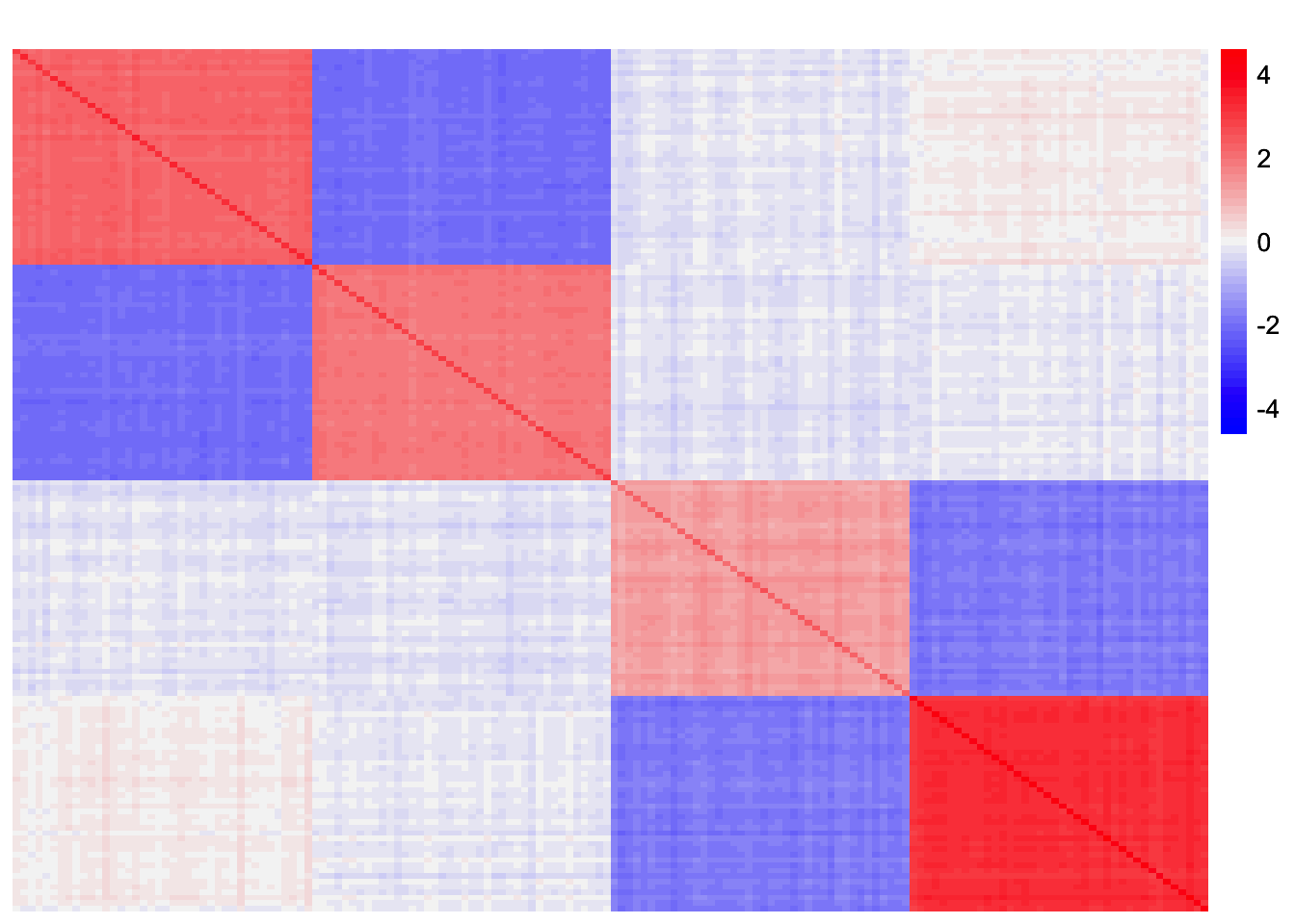

Observations

We see that symEBcovMF with the refitting step does a better job at recovering the hierarchical structure of the data. The loadings estimate does not look entirely binary, but this is to be expected since we used the point-exponential prior. One could imagine a procedure where you start with a fit using point-exponential prior, and then refine the estimates using the generalized binary prior.

I did try symEBcovMF with refitting with the generalized binary factor, and it yields a different representation. The first factor is an intercept like factor and the next two factors are subtype-effect factors. Factor 5 is a population effect factor. However, factors 4, 6, and 7 are not population effects. I think the method found a different representation for the four population effects (which is something I’ve seen in other examples). I’m not sure why the point-exponential prior and the generalized binary prior led to different representations. Perhaps the point-exponential prior is better at yielding sparser solutions? This would also motivate a procedure that uses point-exponential as an initialization and then uses generalized binary to make the loadings more binary.

sessionInfo()

R version 4.3.2 (2023-10-31)
Platform: aarch64-apple-darwin20 (64-bit)
Running under: macOS Sonoma 14.4.1

Matrix products: default
BLAS:   /Library/Frameworks/R.framework/Versions/4.3-arm64/Resources/lib/libRblas.0.dylib 
LAPACK: /Library/Frameworks/R.framework/Versions/4.3-arm64/Resources/lib/libRlapack.dylib;  LAPACK version 3.11.0

locale:
[1] en_US.UTF-8/en_US.UTF-8/en_US.UTF-8/C/en_US.UTF-8/en_US.UTF-8

time zone: America/Chicago
tzcode source: internal

attached base packages:
[1] stats     graphics  grDevices utils     datasets  methods   base     

other attached packages:
[1] ggplot2_3.5.1   pheatmap_1.0.12 ebnm_1.1-34     workflowr_1.7.1

loaded via a namespace (and not attached):
 [1] gtable_0.3.5       xfun_0.48          bslib_0.8.0        processx_3.8.4    
 [5] lattice_0.22-6     callr_3.7.6        vctrs_0.6.5        tools_4.3.2       
 [9] ps_1.7.7           generics_0.1.3     tibble_3.2.1       fansi_1.0.6       
[13] highr_0.11         pkgconfig_2.0.3    Matrix_1.6-5       SQUAREM_2021.1    
[17] RColorBrewer_1.1-3 lifecycle_1.0.4    truncnorm_1.0-9    farver_2.1.2      
[21] compiler_4.3.2     stringr_1.5.1      git2r_0.33.0       munsell_0.5.1     
[25] getPass_0.2-4      httpuv_1.6.15      htmltools_0.5.8.1  sass_0.4.9        
[29] yaml_2.3.10        later_1.3.2        pillar_1.9.0       jquerylib_0.1.4   
[33] whisker_0.4.1      cachem_1.1.0       trust_0.1-8        RSpectra_0.16-2   
[37] tidyselect_1.2.1   digest_0.6.37      stringi_1.8.4      dplyr_1.1.4       
[41] ashr_2.2-66        labeling_0.4.3     splines_4.3.2      rprojroot_2.0.4   
[45] fastmap_1.2.0      grid_4.3.2         colorspace_2.1-1   cli_3.6.3         
[49] invgamma_1.1       magrittr_2.0.3     utf8_1.2.4         withr_3.0.1       
[53] scales_1.3.0       promises_1.3.0     horseshoe_0.2.0    rmarkdown_2.28    
[57] httr_1.4.7         deconvolveR_1.2-1  evaluate_1.0.0     knitr_1.48        
[61] irlba_2.3.5.1      rlang_1.1.4        Rcpp_1.0.13        mixsqp_0.3-54     
[65] glue_1.8.0         rstudioapi_0.16.0  jsonlite_1.8.9     R6_2.5.1          
[69] fs_1.6.4

symebcovmf_tree

Annie Xie

2025-04-08

Introduction

Example

Data Generation

symEBcovMF

Progression of ELBO

Visualization of Estimate

Visualization of Fit

Visualization of Residual Matrix

Observations

symEBcovMF with refit step

Progression of ELBO

Visualization of Estimate

Visualization of Fit

Visualization of Residual Matrix

Observations