symebcovmf_point_exp_init

workflowr

• Summary
• Checks
• Past versions

Last updated: 2025-05-05

Checks: 7 0

Knit directory: symmetric_covariance_decomposition/

This reproducible R Markdown analysis was created with workflowr (version 1.7.1). The Checks tab describes the reproducibility checks that were applied when the results were created. The Past versions tab lists the development history.

---

R Markdown file: up-to-date

Great! Since the R Markdown file has been committed to the Git repository, you know the exact version of the code that produced these results.

Environment: empty

Great job! The global environment was empty. Objects defined in the global environment can affect the analysis in your R Markdown file in unknown ways. For reproduciblity it’s best to always run the code in an empty environment.

Seed: set.seed(20250408)

The command set.seed(20250408) was run prior to running the code in the R Markdown file. Setting a seed ensures that any results that rely on randomness, e.g. subsampling or permutations, are reproducible.

Session information: recorded

Great job! Recording the operating system, R version, and package versions is critical for reproducibility.

Cache: none

Nice! There were no cached chunks for this analysis, so you can be confident that you successfully produced the results during this run.

File paths: relative

Great job! Using relative paths to the files within your workflowr project makes it easier to run your code on other machines.

Repository version: f70efd7

Great! You are using Git for version control. Tracking code development and connecting the code version to the results is critical for reproducibility.

The results in this page were generated with repository version f70efd7. See the Past versions tab to see a history of the changes made to the R Markdown and HTML files.

Note that you need to be careful to ensure that all relevant files for the analysis have been committed to Git prior to generating the results (you can use wflow_publish or wflow_git_commit). workflowr only checks the R Markdown file, but you know if there are other scripts or data files that it depends on. Below is the status of the Git repository when the results were generated:

Ignored files:
    Ignored:    .DS_Store
    Ignored:    .Rhistory

Untracked files:
    Untracked:  analysis/symebcovmf_binary_tree_resid_orthog_exploration.Rmd
    Untracked:  analysis/unbal_nonoverlap_exploration.Rmd

Unstaged changes:
    Modified:   analysis/unbal_nonoverlap.Rmd

Note that any generated files, e.g. HTML, png, CSS, etc., are not included in this status report because it is ok for generated content to have uncommitted changes.

---

These are the previous versions of the repository in which changes were made to the R Markdown (analysis/symebcovmf_point_exp_init.Rmd) and HTML (docs/symebcovmf_point_exp_init.html) files. If you’ve configured a remote Git repository (see ?wflow_git_remote), click on the hyperlinks in the table below to view the files as they were in that past version.

File	Version	Author	Date	Message
Rmd	f70efd7	Annie Xie	2025-05-05	Edit text in point-exponential init analysis
html	484b322	Annie Xie	2025-04-28	Build site.
Rmd	daf1ee3	Annie Xie	2025-04-28	Update point exponential initialization analysis
html	b407abe	Annie Xie	2025-04-21	Build site.
Rmd	f334e30	Annie Xie	2025-04-21	Add exploration of point-exp initialization

---

Introduction

In this analysis, I want to test out initializing symEBcovMF with the generalized binary prior with symEBcovMF fit with a point-exponential prior.

Packages and Functions

library(ebnm)
library(pheatmap)
library(ggplot2)

source('code/visualization_functions.R')
source('code/symebcovmf_functions.R')

Example

To test this procedure, I will apply it to the tree-structured dataset. When testing out symEBcovMF, I found that the estimates from the two priors in the tree setting had the largest difference.

Data Generation

sim_4pops <- function(args) {
  set.seed(args$seed)
  
  n <- sum(args$pop_sizes)
  p <- args$n_genes
  
  FF <- matrix(rnorm(7 * p, sd = rep(args$branch_sds, each = p)), ncol = 7)
  # if (args$constrain_F) {
  #   FF_svd <- svd(FF)
  #   FF <- FF_svd$u
  #   FF <- t(t(FF) * branch_sds * sqrt(p))
  # }
  
  LL <- matrix(0, nrow = n, ncol = 7)
  LL[, 1] <- 1
  LL[, 2] <- rep(c(1, 1, 0, 0), times = args$pop_sizes)
  LL[, 3] <- rep(c(0, 0, 1, 1), times = args$pop_sizes)
  LL[, 4] <- rep(c(1, 0, 0, 0), times = args$pop_sizes)
  LL[, 5] <- rep(c(0, 1, 0, 0), times = args$pop_sizes)
  LL[, 6] <- rep(c(0, 0, 1, 0), times = args$pop_sizes)
  LL[, 7] <- rep(c(0, 0, 0, 1), times = args$pop_sizes)
  
  E <- matrix(rnorm(n * p, sd = args$indiv_sd), nrow = n)
  Y <- LL %*% t(FF) + E
  YYt <- (1/p)*tcrossprod(Y)
  return(list(Y = Y, YYt = YYt, LL = LL, FF = FF, K = ncol(LL)))
}

sim_args = list(pop_sizes = rep(40, 4), n_genes = 1000, branch_sds = rep(2,7), indiv_sd = 1, seed = 1)
sim_data <- sim_4pops(sim_args)

This is a heatmap of the scaled Gram matrix:

plot_heatmap(sim_data$YYt, colors_range = c('blue','gray96','red'), brks = seq(-max(abs(sim_data$YYt)), max(abs(sim_data$YYt)), length.out = 50))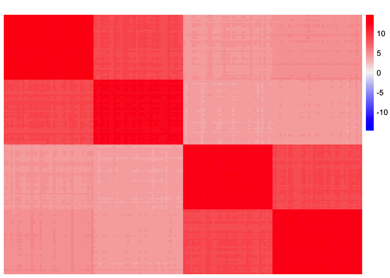

Past versions of unnamed-chunk-5-1.png

Version	Author	Date
b407abe	Annie Xie	2025-04-21

This is a scatter plot of the true loadings matrix:

pop_vec <- c(rep('A', 40), rep('B', 40), rep('C', 40), rep('D', 40))
plot_loadings(sim_data$LL, pop_vec)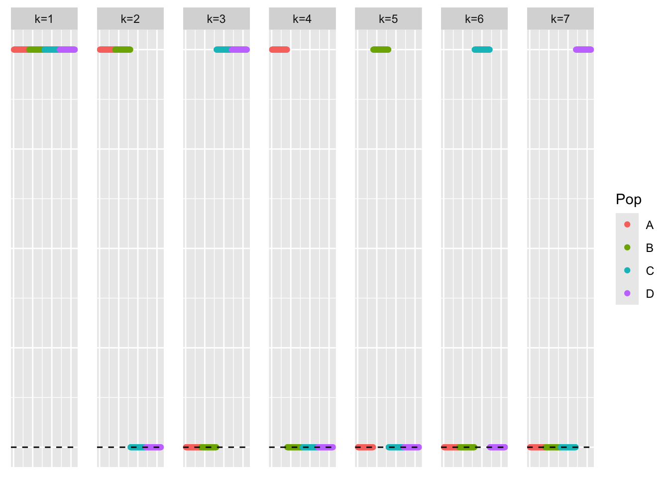

Past versions of unnamed-chunk-6-1.png

Version	Author	Date
b407abe	Annie Xie	2025-04-21

This is a plot of the eigenvalues of the Gram matrix:

S_eigen <- eigen(sim_data$YYt)
plot(S_eigen$values) + abline(a = 0, b = 0, col = 'red')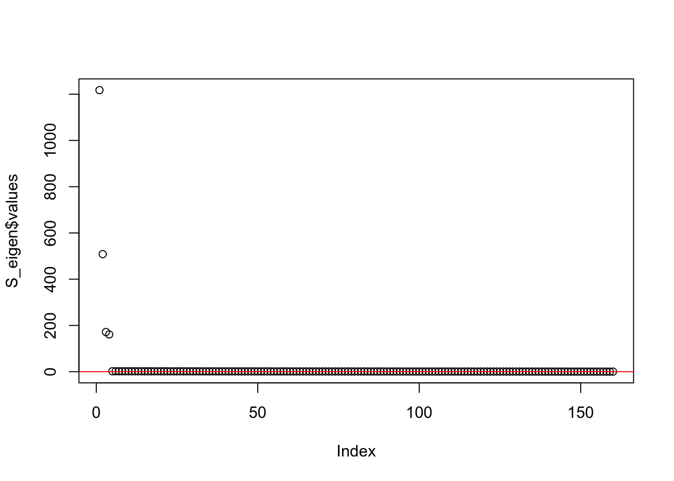

Past versions of unnamed-chunk-7-1.png

Version	Author	Date
b407abe	Annie Xie	2025-04-21

integer(0)

This is the minimum eigenvalue:

min(S_eigen$values)

[1] 0.3724341

Generalized binary symEBcovMF

symebcovmf_fit <- sym_ebcovmf_fit(S = sim_data$YYt, ebnm_fn = ebnm::ebnm_generalized_binary, K = 7, maxiter = 500, rank_one_tol = 10^(-8), tol = 10^(-8), refit_lam = TRUE)

[1] "elbo decreased by 0.185693113584421"
[1] "elbo decreased by 0.0114876429142896"
[1] "elbo decreased by 1.5825207810849e-10"

This is a scatter plot of \(\hat{L}\), the estimate from symEBcovMF:

bal_pops <- c(rep('A', 40), rep('B', 40), rep('C', 40), rep('D', 40))
plot_loadings(symebcovmf_fit$L_pm %*% diag(sqrt(symebcovmf_fit$lambda)), bal_pops)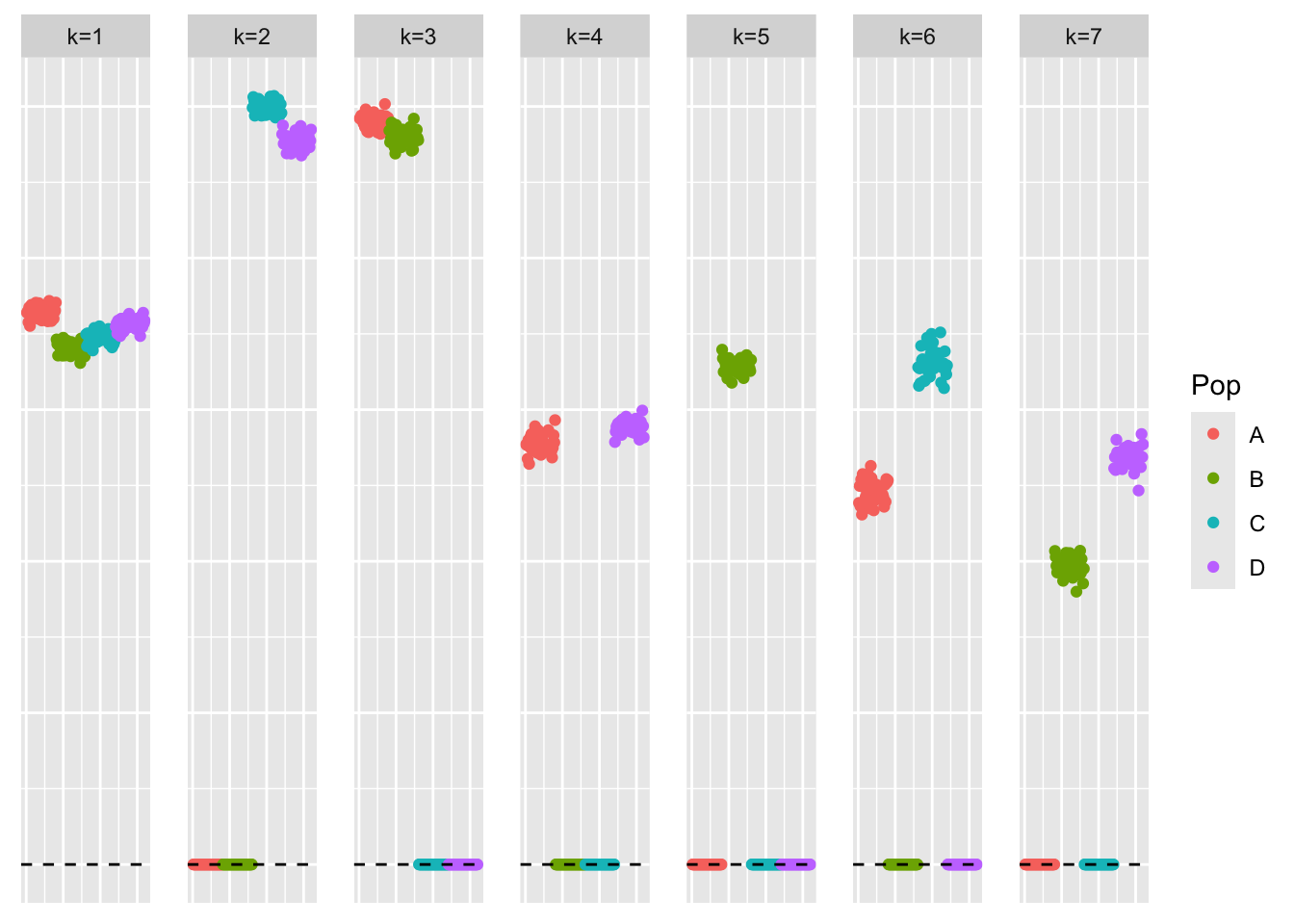

Past versions of unnamed-chunk-10-1.png

Version	Author	Date
b407abe	Annie Xie	2025-04-21

symebcovmf_fit$elbo

[1] -14979.17

Generalized binary symEBcovMF initialized with point-exponential fit

For this procedure, I start by running symEBcovMF with a point-exponential prior with Kmax set to the inputted Kmax value. From this, I get an estimate for \(L\), which I call \(\hat{L}_{exp}\). Then, I run symEBcovMF with a generalized-binary prior. I initialize the rank-one fit for factor \(k\) with the \(k\)-th column of \(\hat{L}_{exp}\). This procedure is a little weird, and I probably will not go with this in the end. Of the options I tried, this was the only one that worked (but there are other options I can try).

sym_ebcovmf_point_exp_init_full_fit <- function(S, ebnm_fn, Kmax, maxiter, rank_one_tol, tol, refit_lam = FALSE){
  #initialize object
  sym_ebcovmf_obj <- sym_ebcovmf_init(S)
  
  symebcovmf_pexp_gb_fit <- sym_ebcovmf_fit(S, ebnm_fn = ebnm::ebnm_point_exponential, K = Kmax, maxiter = maxiter, rank_one_tol = rank_one_tol, tol = tol, refit_lam = refit_lam)
  
  curr_rank <- 0
  obj_diff <- Inf
  while ((curr_rank < Kmax) & (obj_diff > tol)){
    # add factor
    v_init <- symebcovmf_pexp_gb_fit$L_pm[,(curr_rank+1)]
    sym_ebcovmf_obj <- sym_ebcovmf_r1_fit(S, sym_ebcovmf_obj, ebnm_fn, maxiter, rank_one_tol, v_init = v_init)
    
    # check if new factor was added
    if (length(sym_ebcovmf_obj$vec_elbo_K) == curr_rank){
      print(paste('Adding factor', (curr_rank + 1), 'does not improve the objective function'))
      break
    } else {
      if (curr_rank > 0){
        if (refit_lam == TRUE){
          sym_ebcovmf_obj <- refit_lambda(S, sym_ebcovmf_obj)
        }
        obj_diff <- sym_ebcovmf_obj$vec_elbo_K[curr_rank + 1] - sym_ebcovmf_obj$vec_elbo_K[curr_rank]
      }
    }
    curr_rank <- curr_rank + 1
  }
  
  return(sym_ebcovmf_obj)
}

symebcovmf_full_pexp_init_fit <- sym_ebcovmf_point_exp_init_full_fit(S = sim_data$YYt, ebnm_fn = ebnm::ebnm_generalized_binary, K = 7, maxiter = 500, rank_one_tol = 10^(-8), tol = 10^(-8), refit_lam = TRUE)

[1] "elbo decreased by 0.175264992671146"
[1] "elbo decreased by 0.0427249965578085"
[1] "elbo decreased by 0.0834464683030092"
[1] "elbo decreased by 0.0006379234000633"

This is a scatter plot of \(\hat{L}_{exp-init}\), the estimate from symEBcovMF initialized with a point-exponential fit:

bal_pops <- c(rep('A', 40), rep('B', 40), rep('C', 40), rep('D', 40))
plot_loadings(symebcovmf_full_pexp_init_fit$L_pm %*% diag(sqrt(symebcovmf_full_pexp_init_fit$lambda)), bal_pops)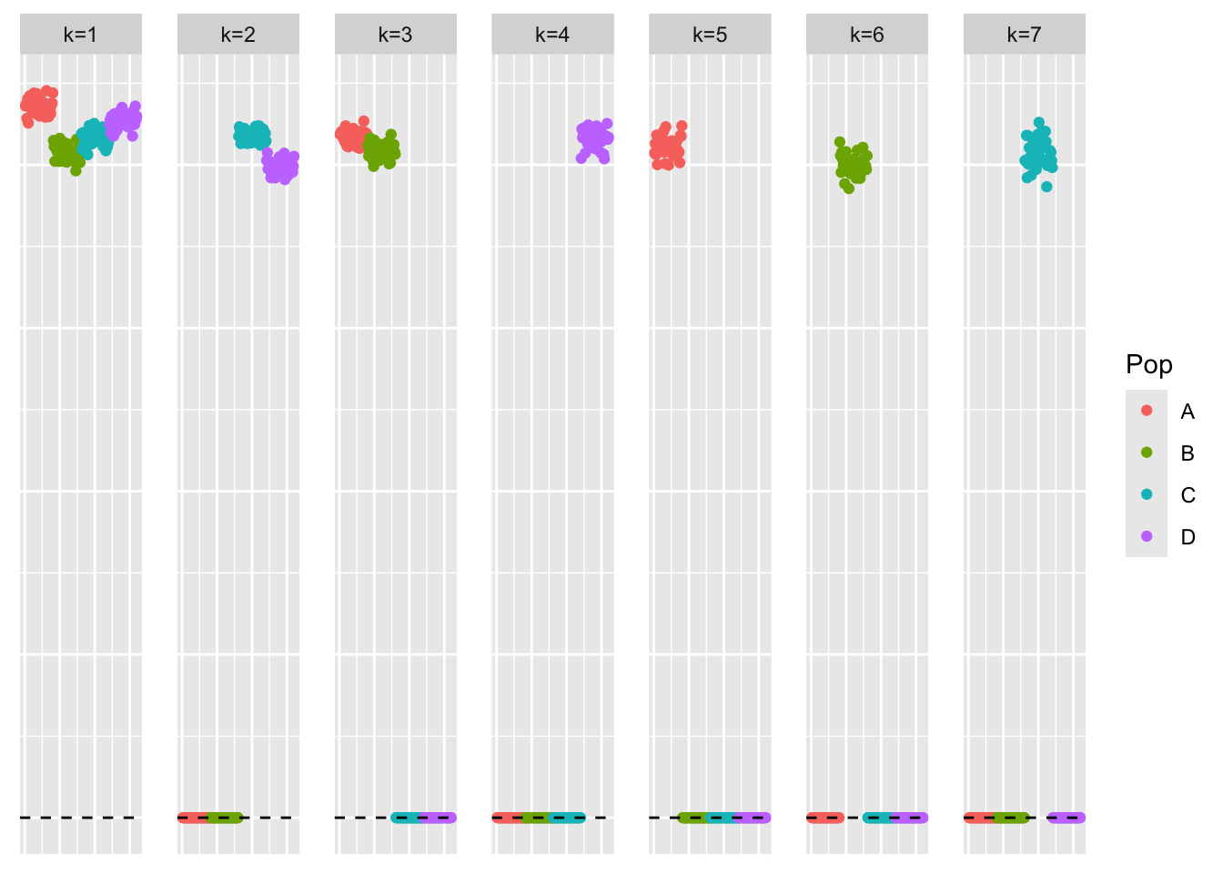

Past versions of unnamed-chunk-14-1.png

Version	Author	Date
b407abe	Annie Xie	2025-04-21

This is the ELBO:

symebcovmf_full_pexp_init_fit$elbo

[1] -7559.355

Comparison

ggplot(data = NULL, aes(x = symebcovmf_fit$L_pm[,1], y = symebcovmf_full_pexp_init_fit$L_pm[,1])) + geom_point() + geom_abline(slope = 1, intercept = 0, color = 'red')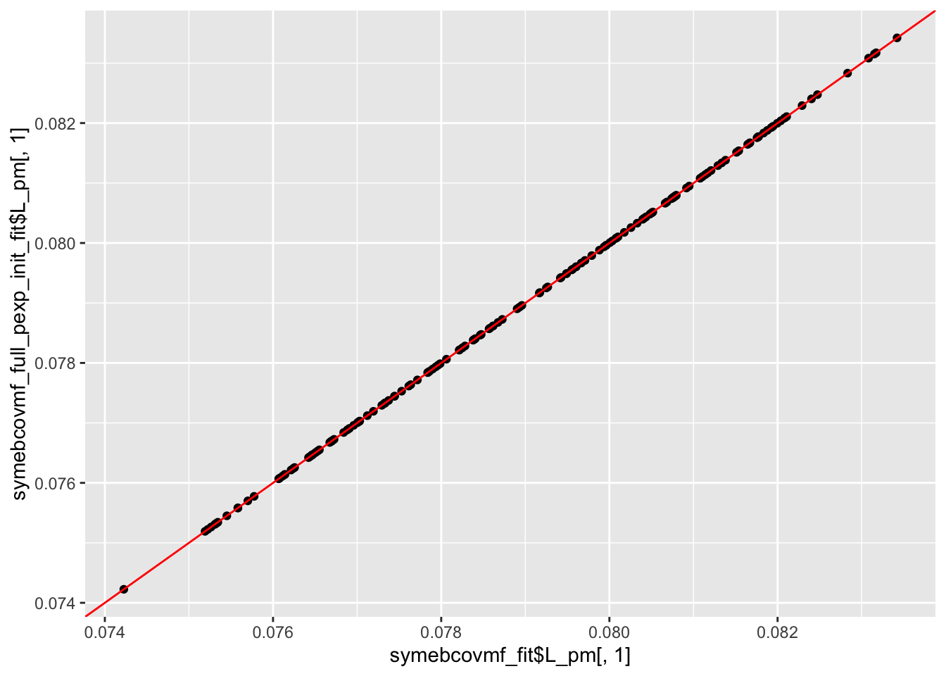

Past versions of unnamed-chunk-16-1.png

Version	Author	Date
484b322	Annie Xie	2025-04-28

ggplot(data = NULL, aes(x = symebcovmf_fit$L_pm[,2], y = symebcovmf_full_pexp_init_fit$L_pm[,2])) + geom_point() + geom_abline(slope = 1, intercept = 0, color = 'red')

Past versions of unnamed-chunk-17-1.png

Version	Author	Date
484b322	Annie Xie	2025-04-28

ggplot(data = NULL, aes(x = symebcovmf_fit$L_pm[,3], y = symebcovmf_full_pexp_init_fit$L_pm[,3])) + geom_point() + geom_abline(slope = 1, intercept = 0, color = 'red')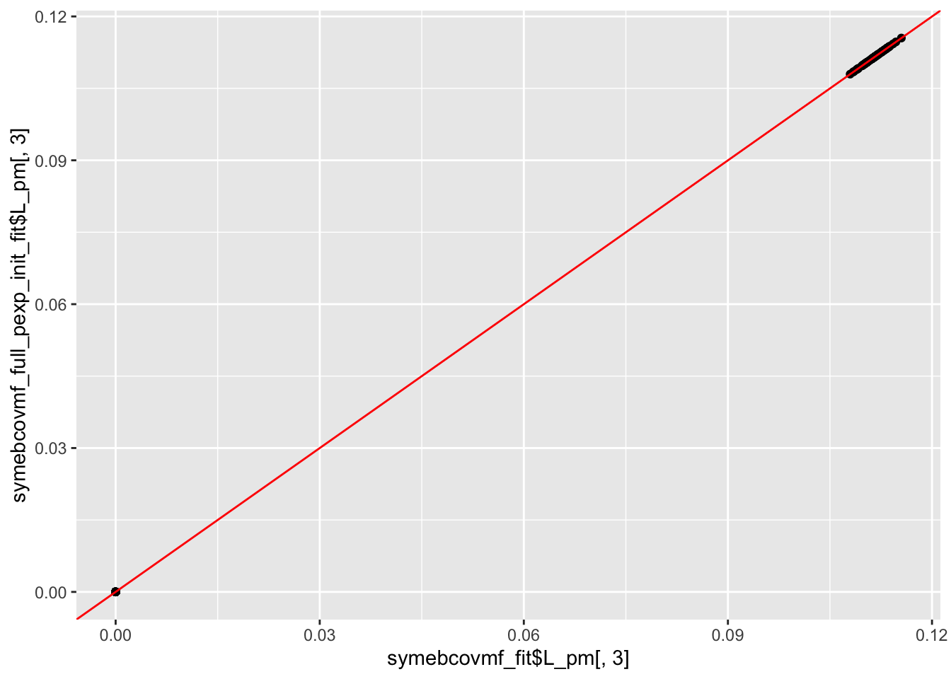

Past versions of unnamed-chunk-18-1.png

Version	Author	Date
484b322	Annie Xie	2025-04-28

Observations

We see that the estimate from generalized binary symEBcovMF initialized with the point-exponential fit looks like a tree, unlike the estimate from generalized binary symEBcovMF initialized with SVD. Furthermore, we see that this estimate obtains a higher ELBO than that of the default method. This suggests that the default method may be getting stuck in a local optima. This is not too surprising. I also suspect that the generalized binary prior is very sensitive to initialization, and may struggle to jump to sparser solutions (even if the sparser solutions yield higher objective function values).

I did try a version of this method where I computed the point-exponential fit for each factor within the rank-one fitting procedure. This point-exponential fit used the current residual matrix computed from factors initialized with point-exponential fits and then refit with generalized binary. However, I found that this method did not yield a tree-like loadings estimate. The estimate looked closer to that of regular generalized binary symEBcovMF. In addition, it only yielded a slightly higher ELBO. I’ve noticed that there are differences in the residual matrices from generalized binary fits vs point-exponential fits. So my best guess for why this occurred is that the residual matrix from the point-exponential fit makes it a little easier to find the group effects one group at a time. Meanwhile, the residual matrix from the generalized binary fit makes it harder to distinguish groups 1 and 4. I explore this more in another analysis. (Perhaps regular power method would also have this issue).

Session information

sessionInfo()

R version 4.3.2 (2023-10-31)
Platform: aarch64-apple-darwin20 (64-bit)
Running under: macOS Sonoma 14.4.1

Matrix products: default
BLAS:   /Library/Frameworks/R.framework/Versions/4.3-arm64/Resources/lib/libRblas.0.dylib 
LAPACK: /Library/Frameworks/R.framework/Versions/4.3-arm64/Resources/lib/libRlapack.dylib;  LAPACK version 3.11.0

locale:
[1] en_US.UTF-8/en_US.UTF-8/en_US.UTF-8/C/en_US.UTF-8/en_US.UTF-8

time zone: America/Chicago
tzcode source: internal

attached base packages:
[1] stats     graphics  grDevices utils     datasets  methods   base     

other attached packages:
[1] ggplot2_3.5.1   pheatmap_1.0.12 ebnm_1.1-34     workflowr_1.7.1

loaded via a namespace (and not attached):
 [1] gtable_0.3.5       xfun_0.48          bslib_0.8.0        processx_3.8.4    
 [5] lattice_0.22-6     callr_3.7.6        vctrs_0.6.5        tools_4.3.2       
 [9] ps_1.7.7           generics_0.1.3     tibble_3.2.1       fansi_1.0.6       
[13] highr_0.11         pkgconfig_2.0.3    Matrix_1.6-5       SQUAREM_2021.1    
[17] RColorBrewer_1.1-3 lifecycle_1.0.4    truncnorm_1.0-9    farver_2.1.2      
[21] compiler_4.3.2     stringr_1.5.1      git2r_0.33.0       munsell_0.5.1     
[25] getPass_0.2-4      httpuv_1.6.15      htmltools_0.5.8.1  sass_0.4.9        
[29] yaml_2.3.10        later_1.3.2        pillar_1.9.0       jquerylib_0.1.4   
[33] whisker_0.4.1      cachem_1.1.0       trust_0.1-8        RSpectra_0.16-2   
[37] tidyselect_1.2.1   digest_0.6.37      stringi_1.8.4      dplyr_1.1.4       
[41] ashr_2.2-66        labeling_0.4.3     splines_4.3.2      rprojroot_2.0.4   
[45] fastmap_1.2.0      grid_4.3.2         colorspace_2.1-1   cli_3.6.3         
[49] invgamma_1.1       magrittr_2.0.3     utf8_1.2.4         withr_3.0.1       
[53] scales_1.3.0       promises_1.3.0     horseshoe_0.2.0    rmarkdown_2.28    
[57] httr_1.4.7         deconvolveR_1.2-1  evaluate_1.0.0     knitr_1.48        
[61] irlba_2.3.5.1      rlang_1.1.4        Rcpp_1.0.13        mixsqp_0.3-54     
[65] glue_1.8.0         rstudioapi_0.16.0  jsonlite_1.8.9     R6_2.5.1          
[69] fs_1.6.4