symebcovmf_laplace_split_init_tree_exploration
Annie Xie
2025-06-19
Last updated: 2025-06-24
Checks: 7 0
Knit directory:
symmetric_covariance_decomposition/
This reproducible R Markdown analysis was created with workflowr (version 1.7.1). The Checks tab describes the reproducibility checks that were applied when the results were created. The Past versions tab lists the development history.
Great! Since the R Markdown file has been committed to the Git repository, you know the exact version of the code that produced these results.
Great job! The global environment was empty. Objects defined in the global environment can affect the analysis in your R Markdown file in unknown ways. For reproduciblity it’s best to always run the code in an empty environment.
The command set.seed(20250408) was run prior to running
the code in the R Markdown file. Setting a seed ensures that any results
that rely on randomness, e.g. subsampling or permutations, are
reproducible.
Great job! Recording the operating system, R version, and package versions is critical for reproducibility.
Nice! There were no cached chunks for this analysis, so you can be confident that you successfully produced the results during this run.
Great job! Using relative paths to the files within your workflowr project makes it easier to run your code on other machines.
Great! You are using Git for version control. Tracking code development and connecting the code version to the results is critical for reproducibility.
The results in this page were generated with repository version 0192295. See the Past versions tab to see a history of the changes made to the R Markdown and HTML files.
Note that you need to be careful to ensure that all relevant files for
the analysis have been committed to Git prior to generating the results
(you can use wflow_publish or
wflow_git_commit). workflowr only checks the R Markdown
file, but you know if there are other scripts or data files that it
depends on. Below is the status of the Git repository when the results
were generated:
Ignored files:
    Ignored:    .DS_Store
    Ignored:    .Rhistory
Note that any generated files, e.g. HTML, png, CSS, etc., are not included in this status report because it is ok for generated content to have uncommitted changes.
These are the previous versions of the repository in which changes were
made to the R Markdown
(analysis/symebcovmf_laplace_split_init_tree_exploration.Rmd)
and HTML
(docs/symebcovmf_laplace_split_init_tree_exploration.html)
files. If you’ve configured a remote Git repository (see
?wflow_git_remote), click on the hyperlinks in the table
below to view the files as they were in that past version.
| File | Version | Author | Date | Message |
|---|---|---|---|---|
| Rmd | 0192295 | Annie Xie | 2025-06-24 | Add further exploration of point laplace splitting init |
Introduction
In this analysis, I further explore the point-Laplace plus splitting initialization strategy for symEBcovMF in the tree setting.
Packages and Functions
library(ebnm)
library(pheatmap)
library(ggplot2)
source('code/visualization_functions.R')
source('code/symebcovmf_functions.R')compute_crossprod_similarity <- function(est, truth){
K_est <- ncol(est)
K_truth <- ncol(truth)
n <- nrow(est)
#if estimates don't have same number of columns, try padding the estimate with zeros and make cosine similarity zero
if (K_est < K_truth){
est <- cbind(est, matrix(rep(0, n*(K_truth-K_est)), nrow = n))
}
if (K_est > K_truth){
truth <- cbind(truth, matrix(rep(0, n*(K_est - K_truth)), nrow = n))
}
#normalize est and truth
norms_est <- apply(est, 2, function(x){sqrt(sum(x^2))})
norms_est[norms_est == 0] <- Inf
norms_truth <- apply(truth, 2, function(x){sqrt(sum(x^2))})
norms_truth[norms_truth == 0] <- Inf
est_normalized <- t(t(est)/norms_est)
truth_normalized <- t(t(truth)/norms_truth)
#compute matrix of cosine similarities
cosine_sim_matrix <- abs(crossprod(est_normalized, truth_normalized))
assignment_problem <- lpSolve::lp.assign(t(cosine_sim_matrix), direction = "max")
return((1/K_truth)*assignment_problem$objval)
}Backfit Functions
optimize_factor <- function(R, ebnm_fn, maxiter, tol, v_init, lambda_k, R2k, n, KL){
  R2 <- R2k - lambda_k^2
  resid_s2 <- estimate_resid_s2(n = n, R2 = R2)
  rank_one_KL <- 0
  curr_elbo <- -Inf
  obj_diff <- Inf
  fitted_g_k <- NULL
  iter <- 1
  vec_elbo_full <- NULL
  v <- v_init

  while((iter <= maxiter) && (obj_diff > tol)){
    # update l; power iteration step
    v.old <- v
    x <- R %*% v
    e <- ebnm_fn(x = x, s = sqrt(resid_s2), g_init = fitted_g_k)
    scaling_factor <- sqrt(sum(e$posterior$mean^2) + sum(e$posterior$sd^2))
    if (scaling_factor == 0){ # check if scaling factor is zero
      scaling_factor <- Inf
      v <- e$posterior$mean/scaling_factor
      print('Warning: scaling factor is zero')
      break
    }
    v <- e$posterior$mean/scaling_factor

    # update lambda and R2
    lambda_k.old <- lambda_k
    lambda_k <- max(as.numeric(t(v) %*% R %*% v), 0)
    R2 <- R2k - lambda_k^2

    #store estimate for g
    fitted_g_k.old <- fitted_g_k
    fitted_g_k <- e$fitted_g

    # store KL
    rank_one_KL.old <- rank_one_KL
    rank_one_KL <- as.numeric(e$log_likelihood) +
      - normal_means_loglik(x, sqrt(resid_s2), e$posterior$mean, e$posterior$mean^2 + e$posterior$sd^2)

    # update resid_s2
    resid_s2.old <- resid_s2
    resid_s2 <- estimate_resid_s2(n = n, R2 = R2) # this goes negative?????

    # check convergence - maybe change to rank-one obj function
    curr_elbo.old <- curr_elbo
    curr_elbo <- compute_elbo(resid_s2 = resid_s2,
                              n = n,
                              KL = c(KL, rank_one_KL),
                              R2 = R2)
    if (iter > 1){
      obj_diff <- curr_elbo - curr_elbo.old
    }
    if (obj_diff < 0){ # check if convergence_val < 0
      v <- v.old
      resid_s2 <- resid_s2.old
      rank_one_KL <- rank_one_KL.old
      lambda_k <- lambda_k.old
      curr_elbo <- curr_elbo.old
      fitted_g_k <- fitted_g_k.old
      print(paste('elbo decreased by', abs(obj_diff)))
      break
    }
    vec_elbo_full <- c(vec_elbo_full, curr_elbo)
    iter <- iter + 1
  }
  return(list(v = v, lambda_k = lambda_k, resid_s2 = resid_s2, curr_elbo = curr_elbo, vec_elbo_full = vec_elbo_full, fitted_g_k = fitted_g_k, rank_one_KL = rank_one_KL))
}
#nullcheck function
nullcheck_factors <- function(sym_ebcovmf_obj, L2_tol = 10^(-8)){
null_lambda_idx <- which(sym_ebcovmf_obj$lambda == 0)
factor_L2_norms <- apply(sym_ebcovmf_obj$L_pm, 2, function(v){sqrt(sum(v^2))})
null_factor_idx <- which(factor_L2_norms < L2_tol)
null_idx <- unique(c(null_lambda_idx, null_factor_idx))
keep_idx <- setdiff(c(1:length(sym_ebcovmf_obj$lambda)), null_idx)
if (length(keep_idx) < length(sym_ebcovmf_obj$lambda)){
#remove factors
sym_ebcovmf_obj$L_pm <- sym_ebcovmf_obj$L_pm[,keep_idx]
sym_ebcovmf_obj$lambda <- sym_ebcovmf_obj$lambda[keep_idx]
sym_ebcovmf_obj$KL <- sym_ebcovmf_obj$KL[keep_idx]
sym_ebcovmf_obj$fitted_gs <- sym_ebcovmf_obj$fitted_gs[keep_idx]
}
#shouldn't need to recompute objective function or other things
return(sym_ebcovmf_obj)
}sym_ebcovmf_backfit <- function(S, sym_ebcovmf_obj, ebnm_fn, backfit_maxiter = 100, backfit_tol = 10^(-8), optim_maxiter= 500, optim_tol = 10^(-8)){
K <- length(sym_ebcovmf_obj$lambda)
iter <- 1
obj_diff <- Inf
sym_ebcovmf_obj$backfit_vec_elbo_full <- NULL
sym_ebcovmf_obj$backfit_iter_elbo_vec <- NULL
# refit lambda
sym_ebcovmf_obj <- refit_lambda(S, sym_ebcovmf_obj, maxiter = 25)
while((iter <= backfit_maxiter) && (obj_diff > backfit_tol)){
# print(iter)
obj_old <- sym_ebcovmf_obj$elbo
# loop through each factor
for (k in 1:K){
# print(k)
# compute residual matrix
R <- S - tcrossprod(sym_ebcovmf_obj$L_pm[,-k] %*% diag(sqrt(sym_ebcovmf_obj$lambda[-k]), ncol = (K-1)))
R2k <- compute_R2(S, sym_ebcovmf_obj$L_pm[,-k], sym_ebcovmf_obj$lambda[-k], (K-1)) #this is right but I have one instance where the values don't match what I expect
# optimize factor
factor_proposed <- optimize_factor(R, ebnm_fn, optim_maxiter, optim_tol, sym_ebcovmf_obj$L_pm[,k], sym_ebcovmf_obj$lambda[k], R2k, sym_ebcovmf_obj$n, sym_ebcovmf_obj$KL[-k])
# update object
sym_ebcovmf_obj$L_pm[,k] <- factor_proposed$v
sym_ebcovmf_obj$KL[k] <- factor_proposed$rank_one_KL
sym_ebcovmf_obj$lambda[k] <- factor_proposed$lambda_k
sym_ebcovmf_obj$resid_s2 <- factor_proposed$resid_s2
sym_ebcovmf_obj$fitted_gs[[k]] <- factor_proposed$fitted_g_k
sym_ebcovmf_obj$elbo <- factor_proposed$curr_elbo
sym_ebcovmf_obj$backfit_vec_elbo_full <- c(sym_ebcovmf_obj$backfit_vec_elbo_full, factor_proposed$vec_elbo_full)
#print(sym_ebcovmf_obj$elbo)
sym_ebcovmf_obj <- refit_lambda(S, sym_ebcovmf_obj) # add refitting step?
#print(sym_ebcovmf_obj$elbo)
}
sym_ebcovmf_obj$backfit_iter_elbo_vec <- c(sym_ebcovmf_obj$backfit_iter_elbo_vec, sym_ebcovmf_obj$elbo)
iter <- iter + 1
obj_diff <- abs(sym_ebcovmf_obj$elbo - obj_old)
# need to add check if it is negative?
}
# nullcheck
sym_ebcovmf_obj <- nullcheck_factors(sym_ebcovmf_obj)
return(sym_ebcovmf_obj)
}Data Generation
To test this procedure, I will apply it to the tree-structured dataset.
sim_4pops <- function(args) {
  set.seed(args$seed)

  n <- sum(args$pop_sizes)
  p <- args$n_genes

  FF <- matrix(rnorm(7 * p, sd = rep(args$branch_sds, each = p)), ncol = 7)
  # if (args$constrain_F) {
  #   FF_svd <- svd(FF)
  #   FF <- FF_svd$u
  #   FF <- t(t(FF) * branch_sds * sqrt(p))
  # }

  LL <- matrix(0, nrow = n, ncol = 7)
  LL[, 1] <- 1
  LL[, 2] <- rep(c(1, 1, 0, 0), times = args$pop_sizes)
  LL[, 3] <- rep(c(0, 0, 1, 1), times = args$pop_sizes)
  LL[, 4] <- rep(c(1, 0, 0, 0), times = args$pop_sizes)
  LL[, 5] <- rep(c(0, 1, 0, 0), times = args$pop_sizes)
  LL[, 6] <- rep(c(0, 0, 1, 0), times = args$pop_sizes)
  LL[, 7] <- rep(c(0, 0, 0, 1), times = args$pop_sizes)

  E <- matrix(rnorm(n * p, sd = args$indiv_sd), nrow = n)
  Y <- LL %*% t(FF) + E
  YYt <- (1/p)*tcrossprod(Y)
  return(list(Y = Y, YYt = YYt, LL = LL, FF = FF, K = ncol(LL)))
}
sim_args = list(pop_sizes = rep(40, 4), n_genes = 1000, branch_sds = rep(2,7), indiv_sd = 1, seed = 1)
sim_data <- sim_4pops(sim_args)This is a heatmap of the scaled Gram matrix:
plot_heatmap(sim_data$YYt, colors_range = c('blue','gray96','red'), brks = seq(-max(abs(sim_data$YYt)), max(abs(sim_data$YYt)), length.out = 50))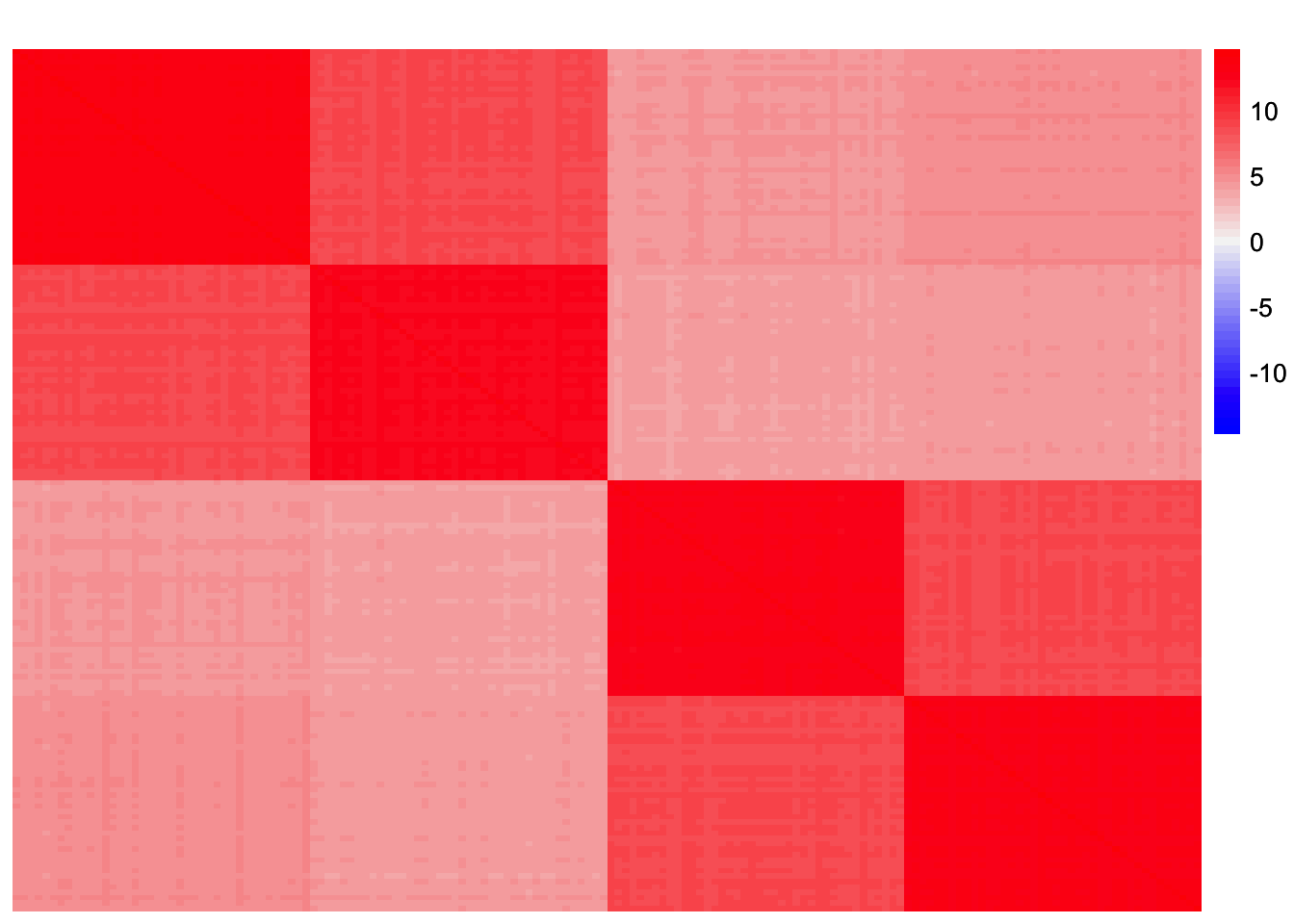
This is a scatter plot of the true loadings matrix:
pop_vec <- c(rep('A', 40), rep('B', 40), rep('C', 40), rep('D', 40))
plot_loadings(sim_data$LL, pop_vec)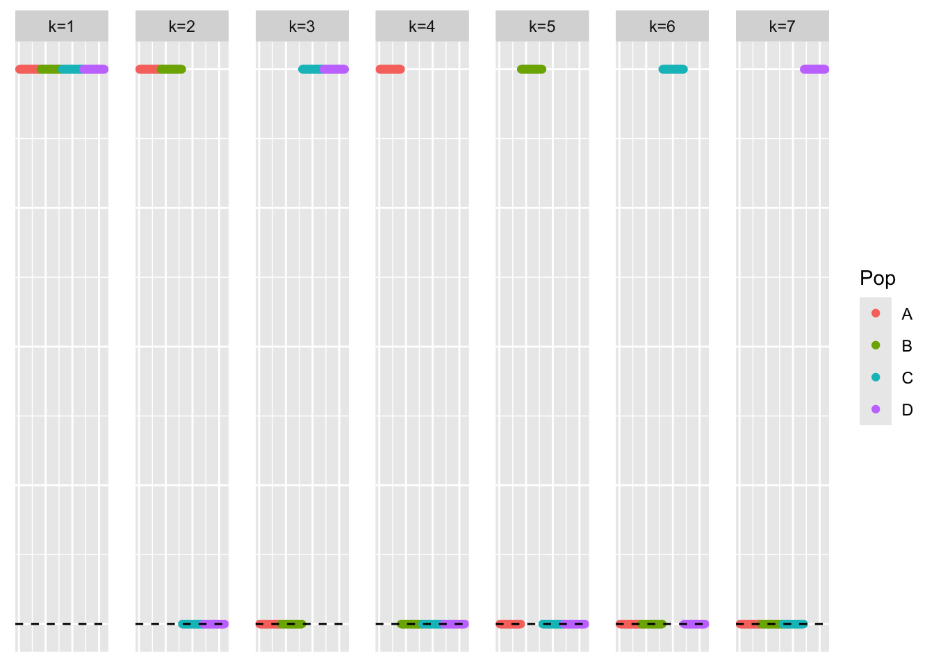
This is a plot of the eigenvalues of the Gram matrix:
S_eigen <- eigen(sim_data$YYt)
plot(S_eigen$values) + abline(a = 0, b = 0, col = 'red')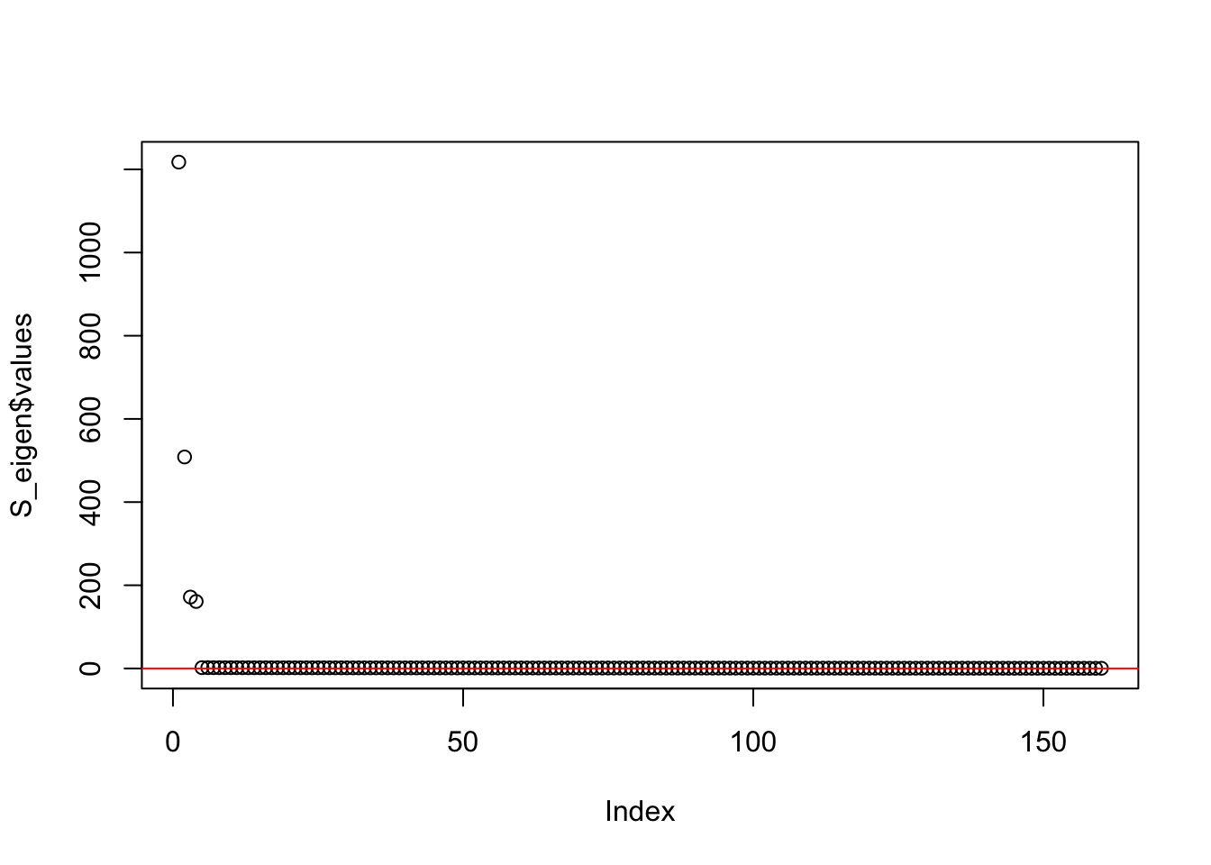
integer(0)This is the minimum eigenvalue:
min(S_eigen$values)[1] 0.3724341Split point-Laplace Fit
I will load in previously saved results for the point-Laplace fit:
symebcovmf_laplace_fit <- readRDS('data/symebcovmf_laplace_tree_backfit_20000.rds')Now, we split the estimate into its positive and negative parts.
LL_split_init <- cbind(pmax(symebcovmf_laplace_fit$L_pm, 0), pmax(-symebcovmf_laplace_fit$L_pm, 0))This is a plot of the estimate with its positive and negative parts split into different factors, \(\hat{L}_{split}\).
plot_loadings(LL_split_init, pop_vec)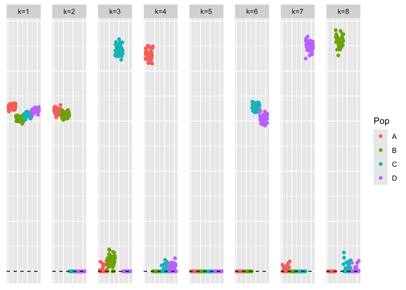
This is a heatmap of the estimate with its positive and negative parts split into different factors, \(\hat{L}_{split}\).
plot_heatmap(LL_split_init)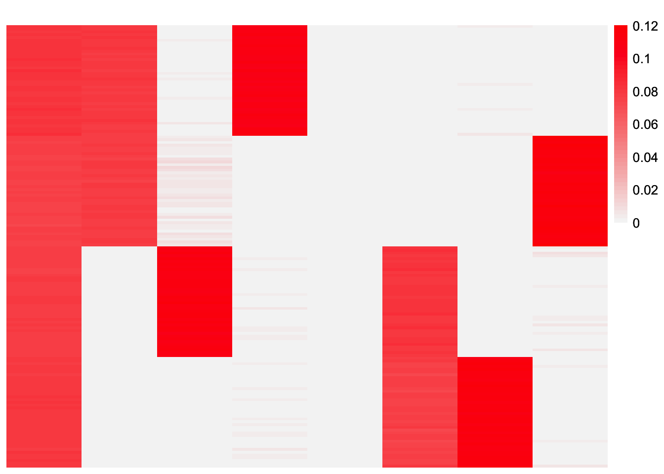
Backfit with Split Initialization
Now, we backfit from the split initialization (this is what GBCD does). The backfit is run with the point-exponential prior.
First, we initialize a symEBcovMF object using \(\hat{L}_{split}\).
symebcovmf_laplace_split_init_obj <- sym_ebcovmf_init(sim_data$YYt)

split_L_norms <- apply(LL_split_init, 2, function(x){sqrt(sum(x^2))})
idx.keep <- which(split_L_norms > 0)
split_L_normalized <- apply(LL_split_init[,idx.keep], 2, function(x){x/sqrt(sum(x^2))})
symebcovmf_laplace_split_init_obj$L_pm <- split_L_normalized

symebcovmf_laplace_split_init_obj$lambda <- rep(symebcovmf_laplace_fit$lambda, times = 2)[idx.keep]

symebcovmf_laplace_split_init_obj$resid_s2 <- estimate_resid_s2(S = sim_data$YYt,
  L = symebcovmf_laplace_split_init_obj$L_pm,
  lambda = symebcovmf_laplace_split_init_obj$lambda,
  n = nrow(sim_data$Y),
  K = length(symebcovmf_laplace_split_init_obj$lambda))

symebcovmf_laplace_split_init_obj$elbo <- compute_elbo(S = sim_data$YYt,
  L = symebcovmf_laplace_split_init_obj$L_pm,
  lambda = symebcovmf_laplace_split_init_obj$lambda,
  resid_s2 = symebcovmf_laplace_split_init_obj$resid_s2,
  n = nrow(sim_data$Y),
  K = length(symebcovmf_laplace_split_init_obj$lambda),
  KL = rep(0, length(symebcovmf_laplace_split_init_obj$lambda)))
I refit the lambda values keeping the factors fixed.
# need to check this
symebcovmf_laplace_split_obj <- refit_lambda(S = sim_data$YYt, symebcovmf_laplace_split_init_obj, maxiter = 500)
This is a plot of the initial loadings estimate:
plot_loadings(symebcovmf_laplace_split_init_obj$L_pm %*% diag(sqrt(symebcovmf_laplace_split_init_obj$lambda)), pop_vec)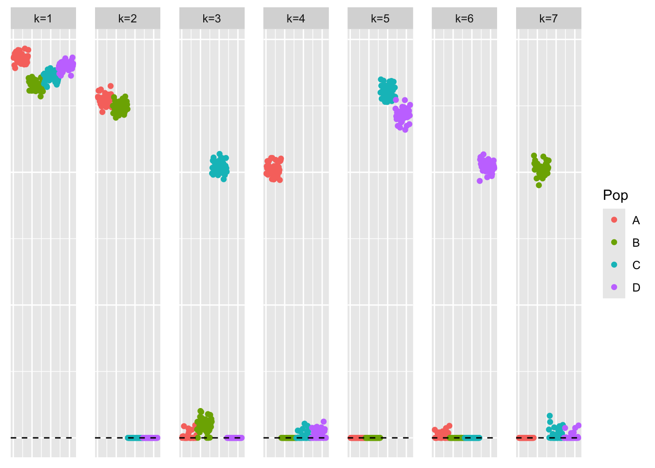
This is a plot of the initial estimate of the scaled Gram matrix:
plot_heatmap(tcrossprod(symebcovmf_laplace_split_init_obj$L_pm %*% diag(sqrt(symebcovmf_laplace_split_init_obj$lambda))), brks = seq(0, max(abs(tcrossprod(symebcovmf_laplace_split_init_obj$L_pm %*% diag(sqrt(symebcovmf_laplace_split_init_obj$lambda))))), length.out = 50))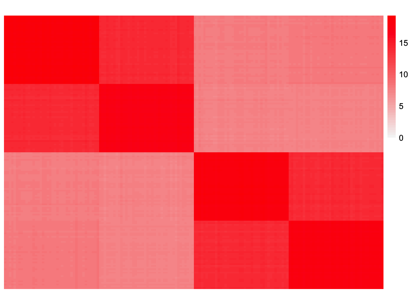
Now, we run the backfit with point-exponential prior.
symebcovmf_laplace_split_init_backfit <- sym_ebcovmf_backfit(sim_data$YYt, symebcovmf_laplace_split_init_obj, ebnm_fn = ebnm::ebnm_point_exponential, backfit_maxiter = 500)This is a plot of the estimate from the backfit initialized with the split estimate, \(\hat{L}_{split-backfit}\).
plot_loadings(symebcovmf_laplace_split_init_backfit$L_pm %*% diag(sqrt(symebcovmf_laplace_split_init_backfit$lambda)), pop_vec)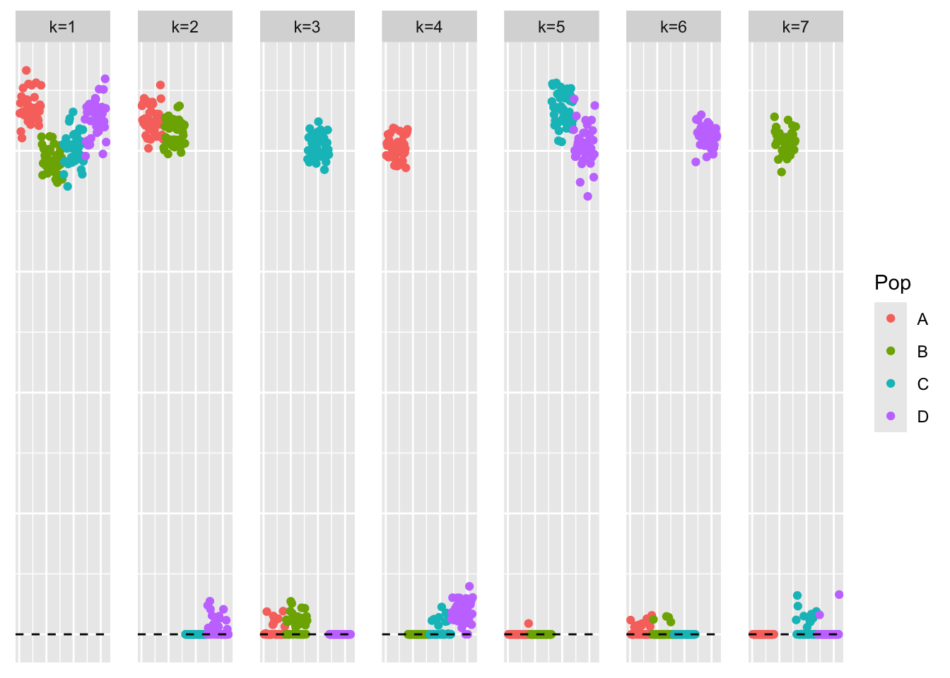
This is a heatmap of the estimate from the backfit initialized with the split estimate, \(\hat{L}_{split-backfit}\).
plot_heatmap(symebcovmf_laplace_split_init_backfit$L_pm %*% diag(sqrt(symebcovmf_laplace_split_init_backfit$lambda)))
This is the crossproduct similarity of the loadings estimate from the backfit initialized with the split estimate, \(\hat{L}_{split-backfit}\).
compute_crossprod_similarity(symebcovmf_laplace_split_init_backfit$L_pm, sim_data$LL)[1] 0.999089This is a heatmap of the estimated Gram matrix, \(\hat{L}_{split-backfit}\hat{\Lambda}\hat{L}_{split-backfit}'\).
gram_est <- tcrossprod(symebcovmf_laplace_split_init_backfit$L_pm %*% diag(sqrt(symebcovmf_laplace_split_init_backfit$lambda)))
plot_heatmap(gram_est, brks = seq(0, max(abs(gram_est)), length.out = 50))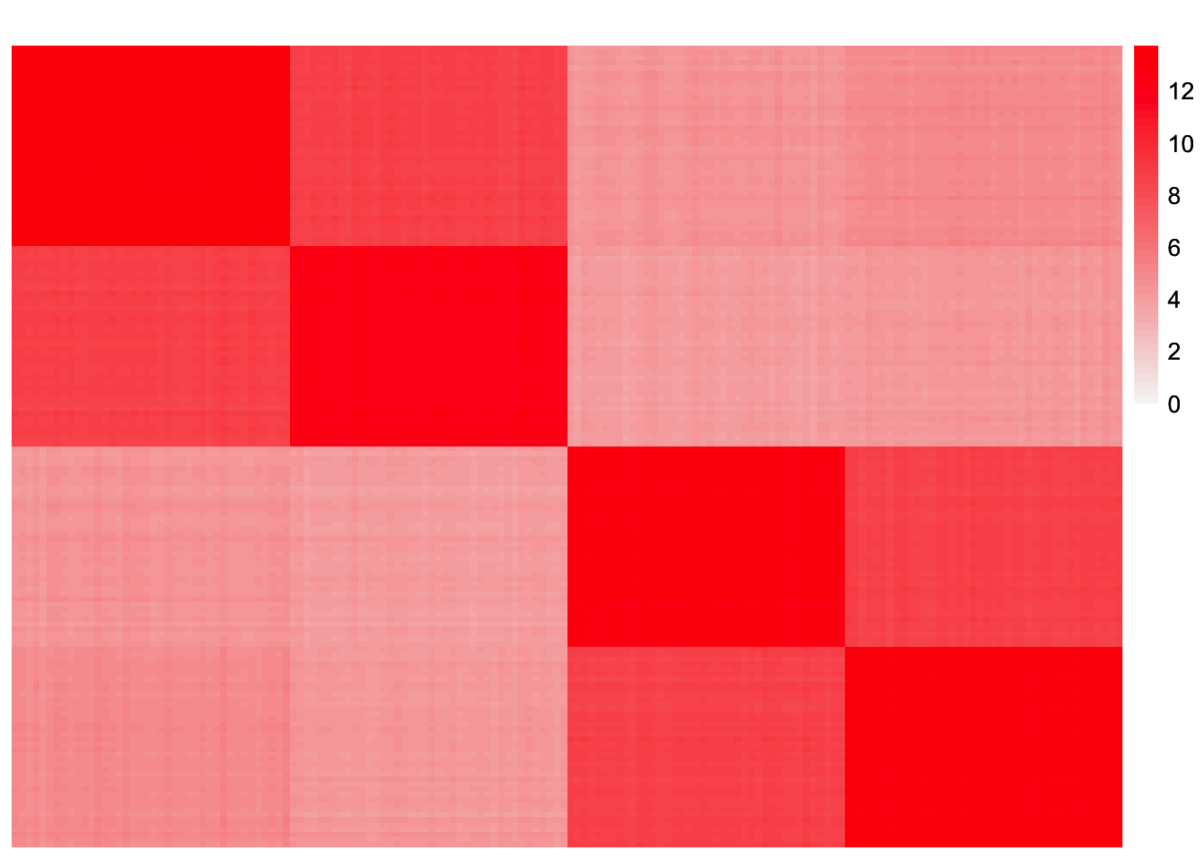
This is the L2 norm of the difference, excluding diagonal entries.
compute_L2_fit <- function(est, dat){
  score <- sum((dat - est)^2) - sum((diag(dat) - diag(est))^2)
  return(score)
}

compute_L2_fit(gram_est, sim_data$YYt)
[1] 30.4981This is a plot of fitted vs. observed values:
ggplot(data = NULL, aes(x = as.vector(sim_data$YYt), y = as.vector(gram_est))) + geom_point() + geom_abline(slope = 1, intercept = 0, color = 'red') + xlab('Observed Values') + ylab('Fitted Values')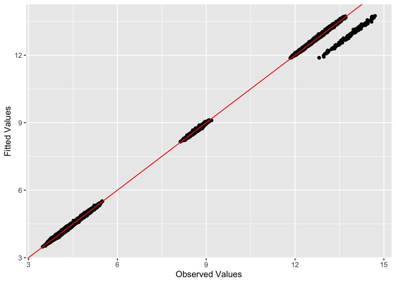
This is a plot of the progression of the ELBO:
plot(symebcovmf_laplace_split_init_backfit$backfit_iter_elbo_vec, ylab = 'ELBO')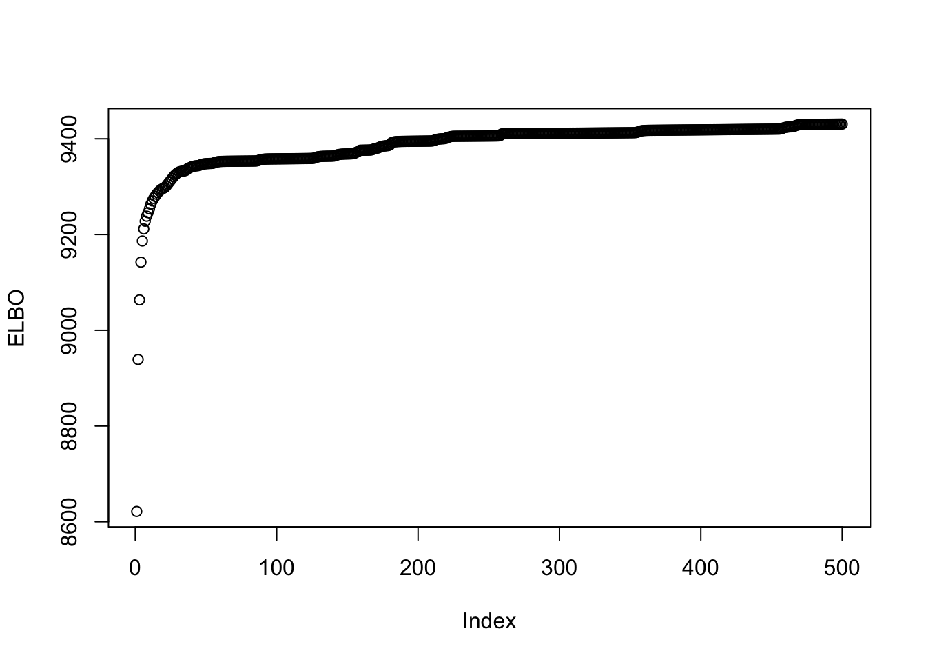
Observations
The estimate from the backfit still captures the tree components and yields a very high crossproduct similarity value. One observation is some of the factors are not fully sparse. For example, in factor 3, which primarily captures the the population effect for population 3, we see that members of populations 1 and 2 now have small non-zero loading. Based on my intuition, I would expect the fully sparse representation to have a higher objective function value, so I’m not exactly sure why these factors have these small loading values in other populations. I imagine these small loading values could be shrunk to zero if you used a binary (or a generalized binary prior that leans toward being binary) to improve the fit.
GBCD
For comparison, I also try applying GBCD with point-exponential prior.
library(gbcd)gbcd_fit <- fit_gbcd(sim_data$Y, Kmax = 7, ebnm::ebnm_point_exponential)[1] "Form cell by cell covariance matrix..."
user system elapsed
0.008 0.000 0.008
[1] "Initialize GEP membership matrix L..."
Adding factor 1 to flash object...
Wrapping up...
Done.
Adding factor 2 to flash object...
Adding factor 3 to flash object...
Adding factor 4 to flash object...
Adding factor 5 to flash object...
Factor doesn't significantly increase objective and won't be added.
Wrapping up...
Done.
Backfitting 4 factors (tolerance: 3.81e-04)...
Difference between iterations is within 1.0e+04...
Difference between iterations is within 1.0e+03...
Difference between iterations is within 1.0e+02...
Difference between iterations is within 1.0e+01...
Difference between iterations is within 1.0e+00...
Difference between iterations is within 1.0e-01...
--Maximum number of iterations reached!
Wrapping up...
Done.
Backfitting 4 factors (tolerance: 3.81e-04)...
Difference between iterations is within 1.0e+03...
Difference between iterations is within 1.0e+02...
Difference between iterations is within 1.0e+01...
Difference between iterations is within 1.0e+00...
Difference between iterations is within 1.0e-01...
Difference between iterations is within 1.0e-02...
Difference between iterations is within 1.0e-03...
Wrapping up...
Done.
Backfitting 4 factors (tolerance: 3.81e-04)...
Difference between iterations is within 1.0e+00...
Wrapping up...
Done.
user system elapsed
3.393 0.071 3.465
[1] "Estimate GEP membership matrix L..."
Backfitting 7 factors (tolerance: 3.81e-04)...
Difference between iterations is within 1.0e+04...
Difference between iterations is within 1.0e+03...
Difference between iterations is within 1.0e+02...
Difference between iterations is within 1.0e+01...
Difference between iterations is within 1.0e+00...
--Maximum number of iterations reached!
Wrapping up...
Done.
Backfitting 7 factors (tolerance: 3.81e-04)...
Difference between iterations is within 1.0e+02...
Difference between iterations is within 1.0e+01...
Difference between iterations is within 1.0e+00...
Difference between iterations is within 1.0e-01...
Difference between iterations is within 1.0e-02...
--Maximum number of iterations reached!
Wrapping up...
Done.
Backfitting 7 factors (tolerance: 3.81e-04)...
Difference between iterations is within 1.0e-01...
Difference between iterations is within 1.0e-02...
--Maximum number of iterations reached!
Wrapping up...
Done.
user system elapsed
6.711 0.085 6.797
[1] "Estimate GEP signature matrix F..."
Backfitting 7 factors (tolerance: 2.38e-03)...
--Estimate of factor 7 is numerically zero!
Difference between iterations is within 1.0e+00...
--Maximum number of iterations reached!
Wrapping up...
Done.
user system elapsed
17.773 0.266 18.047 This is a plot of the loadings estimate from GBCD, \(\hat{L}_{gbcd}\).
plot_loadings(gbcd_fit$L, pop_vec)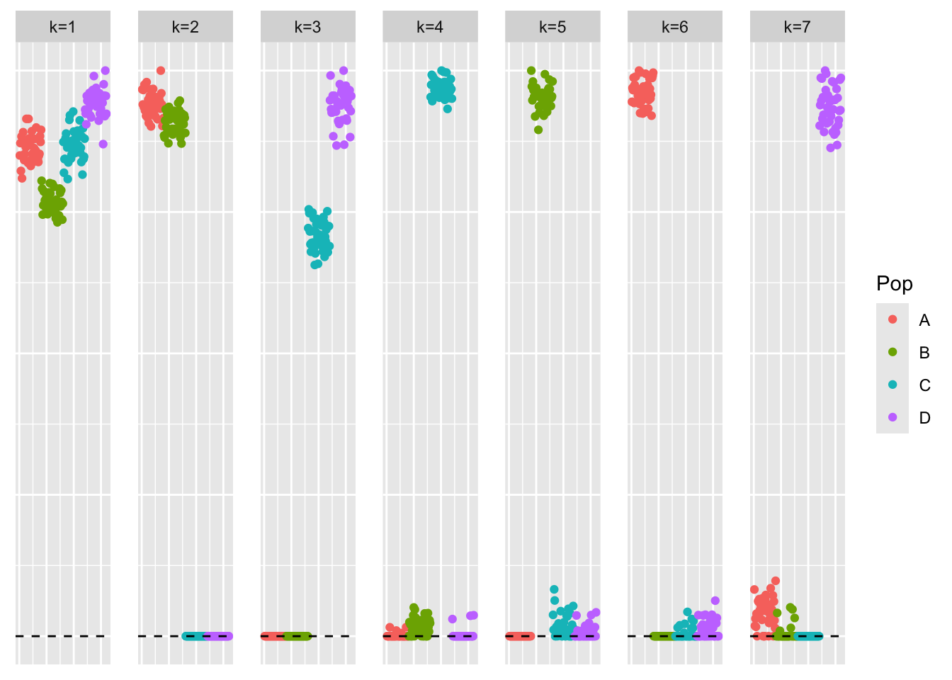
This is a heatmap of the loadings estimate from GBCD, \(\hat{L}_{gbcd}\).
plot_heatmap(gbcd_fit$L)
This is the crossproduct similarity of the loadings estimate from GBCD, \(\hat{L}_{gbcd}\).
compute_crossprod_similarity(gbcd_fit$L, sim_data$LL)[1] 0.9975294Observations
The estimate from GBCD also captures all the tree components and yields a high crossproduct similarity value. The crossproduct similarity is just slightly lower than that of symEBcovMF backfit initialized with the point-Laplace fit plus splitting. We also find that some of the GBCD factors have small non-zero loadings. For example, factor 5, which primarily captures population 2, has small non-zero loadings for members of populations 3 and 4. Given that the GBCD estimate also has this characteristic, I am inclined to think non-zero loadings are a result of model misspecification.
sessionInfo()R version 4.3.2 (2023-10-31)
Platform: aarch64-apple-darwin20 (64-bit)
Running under: macOS 15.4.1
Matrix products: default
BLAS: /Library/Frameworks/R.framework/Versions/4.3-arm64/Resources/lib/libRblas.0.dylib
LAPACK: /Library/Frameworks/R.framework/Versions/4.3-arm64/Resources/lib/libRlapack.dylib; LAPACK version 3.11.0
locale:
[1] en_US.UTF-8/en_US.UTF-8/en_US.UTF-8/C/en_US.UTF-8/en_US.UTF-8
time zone: America/New_York
tzcode source: internal
attached base packages:
[1] stats graphics grDevices utils datasets methods base
other attached packages:
[1] gbcd_0.1-20 ggplot2_3.5.1 pheatmap_1.0.12 ebnm_1.1-34
[5] workflowr_1.7.1
loaded via a namespace (and not attached):
[1] tidyselect_1.2.1 viridisLite_0.4.2 dplyr_1.1.4
[4] farver_2.1.2 fastmap_1.2.0 lazyeval_0.2.2
[7] promises_1.3.0 digest_0.6.37 lifecycle_1.0.4
[10] processx_3.8.4 invgamma_1.1 magrittr_2.0.3
[13] compiler_4.3.2 progress_1.2.3 rlang_1.1.4
[16] sass_0.4.9 tools_4.3.2 utf8_1.2.4
[19] yaml_2.3.10 data.table_1.16.0 knitr_1.48
[22] prettyunits_1.2.0 labeling_0.4.3 htmlwidgets_1.6.4
[25] scatterplot3d_0.3-44 RColorBrewer_1.1-3 Rtsne_0.17
[28] purrr_1.0.2 withr_3.0.1 flashier_1.0.53
[31] grid_4.3.2 fansi_1.0.6 git2r_0.33.0
[34] fastTopics_0.6-192 colorspace_2.1-1 scales_1.3.0
[37] gtools_3.9.5 cli_3.6.3 crayon_1.5.3
[40] rmarkdown_2.28 generics_0.1.3 RcppParallel_5.1.9
[43] rstudioapi_0.16.0 httr_1.4.7 pbapply_1.7-2
[46] cachem_1.1.0 stringr_1.5.1 splines_4.3.2
[49] parallel_4.3.2 softImpute_1.4-1 vctrs_0.6.5
[52] Matrix_1.6-5 jsonlite_1.8.9 callr_3.7.6
[55] hms_1.1.3 mixsqp_0.3-54 ggrepel_0.9.6
[58] irlba_2.3.5.1 horseshoe_0.2.0 trust_0.1-8
[61] plotly_4.10.4 tidyr_1.3.1 jquerylib_0.1.4
[64] glue_1.8.0 ps_1.7.7 uwot_0.1.16
[67] cowplot_1.1.3 stringi_1.8.4 Polychrome_1.5.1
[70] gtable_0.3.5 later_1.3.2 quadprog_1.5-8
[73] munsell_0.5.1 tibble_3.2.1 pillar_1.9.0
[76] htmltools_0.5.8.1 truncnorm_1.0-9 R6_2.5.1
[79] rprojroot_2.0.4 evaluate_1.0.0 lpSolve_5.6.20
[82] lattice_0.22-6 highr_0.11 RhpcBLASctl_0.23-42
[85] SQUAREM_2021.1 ashr_2.2-66 httpuv_1.6.15
[88] bslib_0.8.0 Rcpp_1.0.13 deconvolveR_1.2-1
[91] whisker_0.4.1 xfun_0.48 fs_1.6.4
[94] getPass_0.2-4 pkgconfig_2.0.3