symebcovmf_laplace_model_exploration
Annie Xie
2025-06-12
Last updated: 2025-06-13
Checks: 7 0
Knit directory:
symmetric_covariance_decomposition/
This reproducible R Markdown analysis was created with workflowr (version 1.7.1). The Checks tab describes the reproducibility checks that were applied when the results were created. The Past versions tab lists the development history.
Great! Since the R Markdown file has been committed to the Git repository, you know the exact version of the code that produced these results.
Great job! The global environment was empty. Objects defined in the global environment can affect the analysis in your R Markdown file in unknown ways. For reproduciblity it’s best to always run the code in an empty environment.
The command set.seed(20250408) was run prior to running
the code in the R Markdown file. Setting a seed ensures that any results
that rely on randomness, e.g. subsampling or permutations, are
reproducible.
Great job! Recording the operating system, R version, and package versions is critical for reproducibility.
Nice! There were no cached chunks for this analysis, so you can be confident that you successfully produced the results during this run.
Great job! Using relative paths to the files within your workflowr project makes it easier to run your code on other machines.
Great! You are using Git for version control. Tracking code development and connecting the code version to the results is critical for reproducibility.
The results in this page were generated with repository version e6b02c3. See the Past versions tab to see a history of the changes made to the R Markdown and HTML files.
Note that you need to be careful to ensure that all relevant files for
the analysis have been committed to Git prior to generating the results
(you can use wflow_publish or
wflow_git_commit). workflowr only checks the R Markdown
file, but you know if there are other scripts or data files that it
depends on. Below is the status of the Git repository when the results
were generated:
Ignored files:
    Ignored:    .DS_Store
    Ignored:    .Rhistory
Note that any generated files, e.g. HTML, png, CSS, etc., are not included in this status report because it is ok for generated content to have uncommitted changes.
These are the previous versions of the repository in which changes were
made to the R Markdown
(analysis/symebcovmf_laplace_model_exploration.Rmd) and
HTML (docs/symebcovmf_laplace_model_exploration.html)
files. If you’ve configured a remote Git repository (see
?wflow_git_remote), click on the hyperlinks in the table
below to view the files as they were in that past version.
| File | Version | Author | Date | Message |
|---|---|---|---|---|
| Rmd | e6b02c3 | Annie Xie | 2025-06-13 | Add exploration of greedy symebcovmf in point laplace in tree setting |
Introduction
In this analysis, we explore symEBcovMF with the point-Laplace prior in the tree setting.
Motivation
In previous analyses, I ran greedy-symEBcovMF with the point-Laplace prior in the tree setting, and the method found a non-sparse representation of the data. However, intuitively the sparse representation should have a higher objective function value. I found that for a full four-factor fit, the sparse representation does have a higher objective function value, but when adding each factor, the greedy procedure prefers the non-sparse factors.
In this analysis, I investigate why the greedy method prefers the non-sparse representation. One explanation is the model misspecification. One source of model misspecification is that \(F\) is not exactly orthogonal. Another source of model misspecification is the noise distribution. The symEBcovMF model assumes the Gram matrix is low rank plus normal noise. To generate the data, normal noise is instead added to the data matrix.
Packages and Functions
library(ebnm)
library(pheatmap)
library(ggplot2)
source('code/visualization_functions.R')
source('code/symebcovmf_functions.R')compute_L2_fit <- function(est, dat){
score <- sum((dat - est)^2) - sum((diag(dat) - diag(est))^2)
return(score)
}Data Generation
In this analysis, we work with the tree-structured dataset.
sim_4pops <- function(args) {
  set.seed(args$seed)

  n <- sum(args$pop_sizes)
  p <- args$n_genes

  FF <- matrix(rnorm(7 * p, sd = rep(args$branch_sds, each = p)), ncol = 7)
  if (args$constrain_F) {
    FF_svd <- svd(FF)
    FF <- FF_svd$u
    FF <- t(t(FF) * args$branch_sds * sqrt(p))
  }

  LL <- matrix(0, nrow = n, ncol = 7)
  LL[, 1] <- 1
  LL[, 2] <- rep(c(1, 1, 0, 0), times = args$pop_sizes)
  LL[, 3] <- rep(c(0, 0, 1, 1), times = args$pop_sizes)
  LL[, 4] <- rep(c(1, 0, 0, 0), times = args$pop_sizes)
  LL[, 5] <- rep(c(0, 1, 0, 0), times = args$pop_sizes)
  LL[, 6] <- rep(c(0, 0, 1, 0), times = args$pop_sizes)
  LL[, 7] <- rep(c(0, 0, 0, 1), times = args$pop_sizes)

  E <- matrix(rnorm(n * p, sd = args$indiv_sd), nrow = n)
  Y <- LL %*% t(FF) + E
  YYt <- (1/p)*tcrossprod(Y)
  return(list(Y = Y, YYt = YYt, LL = LL, FF = FF, K = ncol(LL)))
}
sim_args = list(pop_sizes = rep(40, 4), n_genes = 1000, branch_sds = rep(2,7), indiv_sd = 1, seed = 1, constrain_F = FALSE)
sim_data <- sim_4pops(sim_args)This is a heatmap of the scaled Gram matrix:
plot_heatmap(sim_data$YYt, colors_range = c('blue','gray96','red'), brks = seq(-max(abs(sim_data$YYt)), max(abs(sim_data$YYt)), length.out = 50))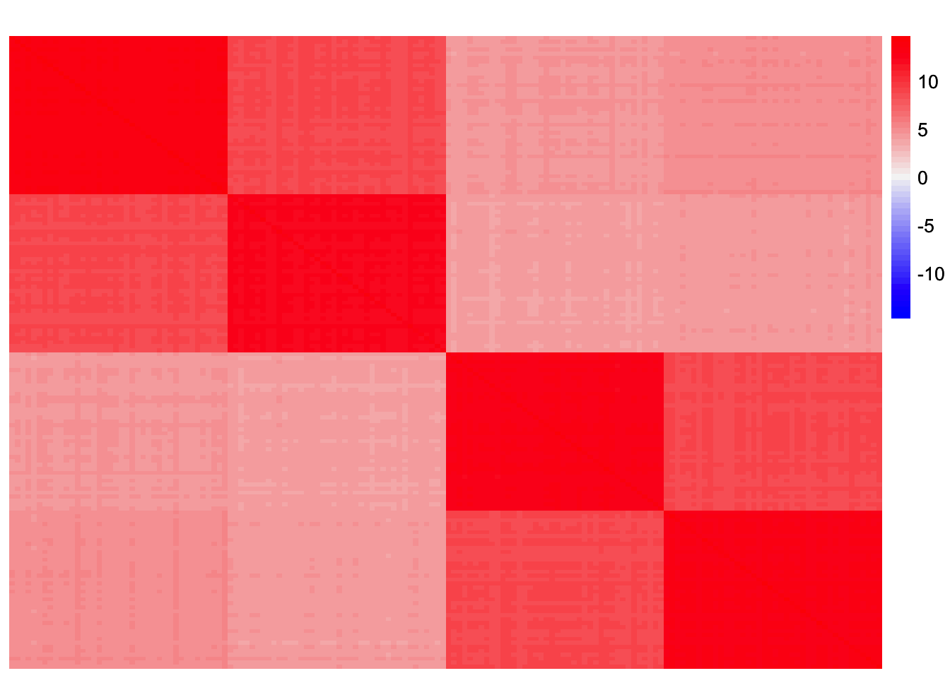
This is a scatter plot of the true loadings matrix:
pop_vec <- c(rep('A', 40), rep('B', 40), rep('C', 40), rep('D', 40))
plot_loadings(sim_data$LL, pop_vec)
This is a plot of the eigenvalues of the Gram matrix:
S_eigen <- eigen(sim_data$YYt)
plot(S_eigen$values) + abline(a = 0, b = 0, col = 'red')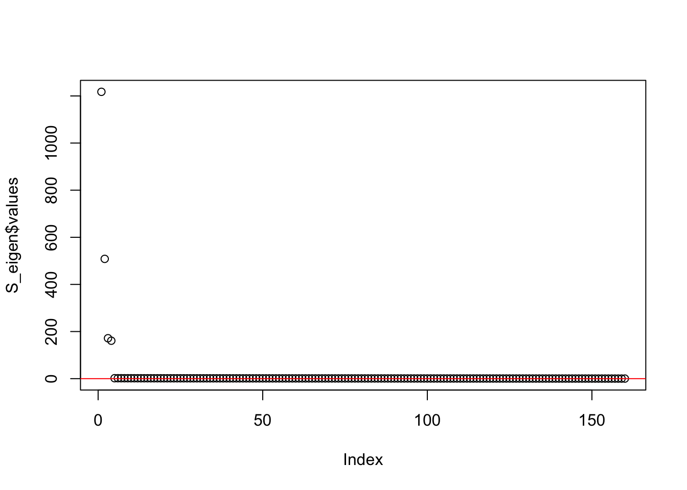
integer(0)This is the minimum eigenvalue:
min(S_eigen$values)[1] 0.3724341symEBcovMF with point-Laplace
First, we start with running greedy symEBcovMF with the point-Laplace prior.
symebcovmf_fit <- sym_ebcovmf_fit(S = sim_data$YYt, ebnm_fn = ebnm::ebnm_point_laplace, K = 7, maxiter = 500, rank_one_tol = 10^(-8), tol = 10^(-8), sign_constraint = NULL, refit_lam = TRUE)[1] "Warning: scaling factor is zero"
[1] "Adding factor 5 does not improve the objective function"This is a scatter plot of \(\hat{L}_{pt-laplace}\), the estimate from symEBcovMF:
bal_pops <- c(rep('A', 40), rep('B', 40), rep('C', 40), rep('D', 40))
plot_loadings(symebcovmf_fit$L_pm %*% diag(sqrt(symebcovmf_fit$lambda)), bal_pops)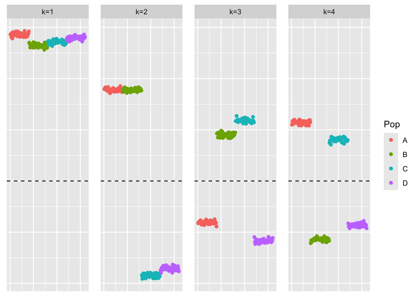
This is the objective function value attained:
symebcovmf_fit$elbo[1] -10362.6Observations
symEBcovMF with point-Laplace prior does not find a divergence factorization. We want the third factor to have zero loading for one branch of populations, and then positive loading for one population and negative loading for the remaining population. We want something analogous for the fourth factor. However, symEBcovMF has found a different third and fourth factor.
Intuitively, the sparser representation should have a higher objective function value due to the sparsity-inducing prior. So we would expect the method to find the sparser representation.
Noiseless case
I consider a setting where we don’t add noise to the data matrix. Thus, \(S = LF'FL'\). If the misspecification of noise is an issue, then I would expect symEBcovMF to get different results in this setting.
symEBcovMF on LF’FL’
YYt_no_noise <- tcrossprod(tcrossprod(sim_data$LL, sim_data$FF))This is a heatmap of the Gram matrix, \(S = LF'FL'\):
plot_heatmap(YYt_no_noise, colors_range = c('blue','gray96','red'), brks = seq(-max(abs(YYt_no_noise)), max(abs(YYt_no_noise)), length.out = 50))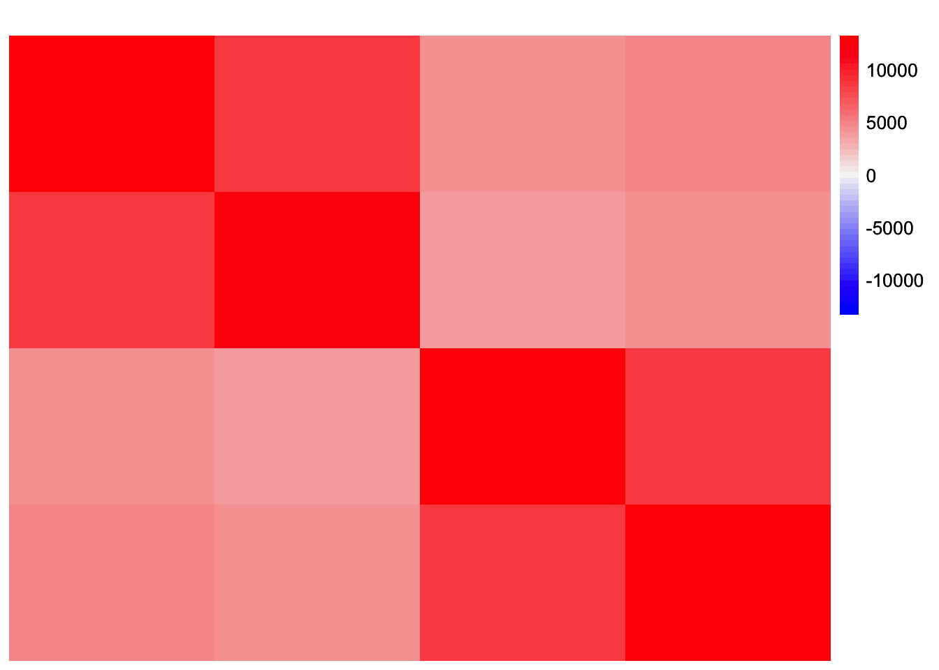
This is a plot of the first four eigenvectors:
YYt_no_noise_eigen <- eigen(YYt_no_noise)
plot_loadings(YYt_no_noise_eigen$vectors[,c(1:4)], bal_pops)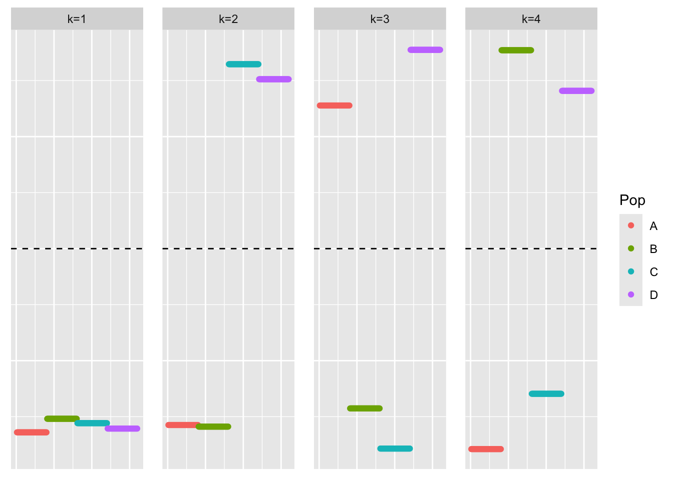
symebcovmf_no_noise_fit <- sym_ebcovmf_fit(S = YYt_no_noise, ebnm_fn = ebnm::ebnm_point_laplace, K = 4, maxiter = 500, rank_one_tol = 10^(-8), tol = 10^(-8), sign_constraint = NULL, refit_lam = TRUE)[1] "elbo decreased by 3.34694050252438e-10"
[1] "elbo decreased by 3.05590219795704e-10"This is a plot of the loadings estimate, \(\hat{L}\):
plot_loadings(symebcovmf_no_noise_fit$L_pm, bal_pops)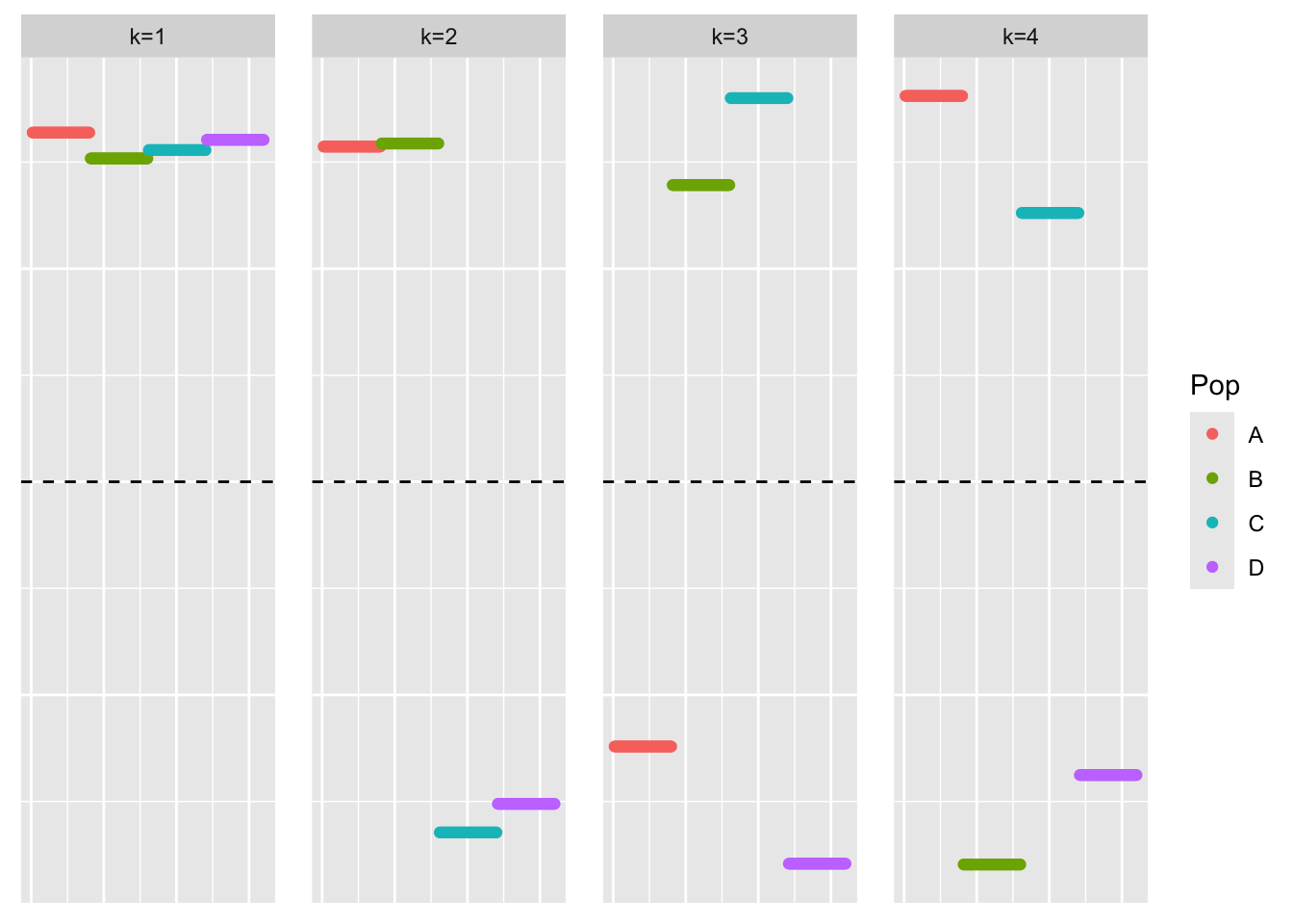
We see that the loadings estimate is still non-sparse.
symEBcovMF on LL’
Now, I want to try running symEBcovMF on \(LL'\) instead, i.e. we are assuming that \(F\) is orthogonal.
YYt_orthog_no_noise <- tcrossprod(sim_data$LL)This is a heatmap of the Gram matrix, \(S = LL'\):
plot_heatmap(YYt_orthog_no_noise, colors_range = c('blue','gray96','red'), brks = seq(-max(abs(YYt_orthog_no_noise)), max(abs(YYt_orthog_no_noise)), length.out = 50))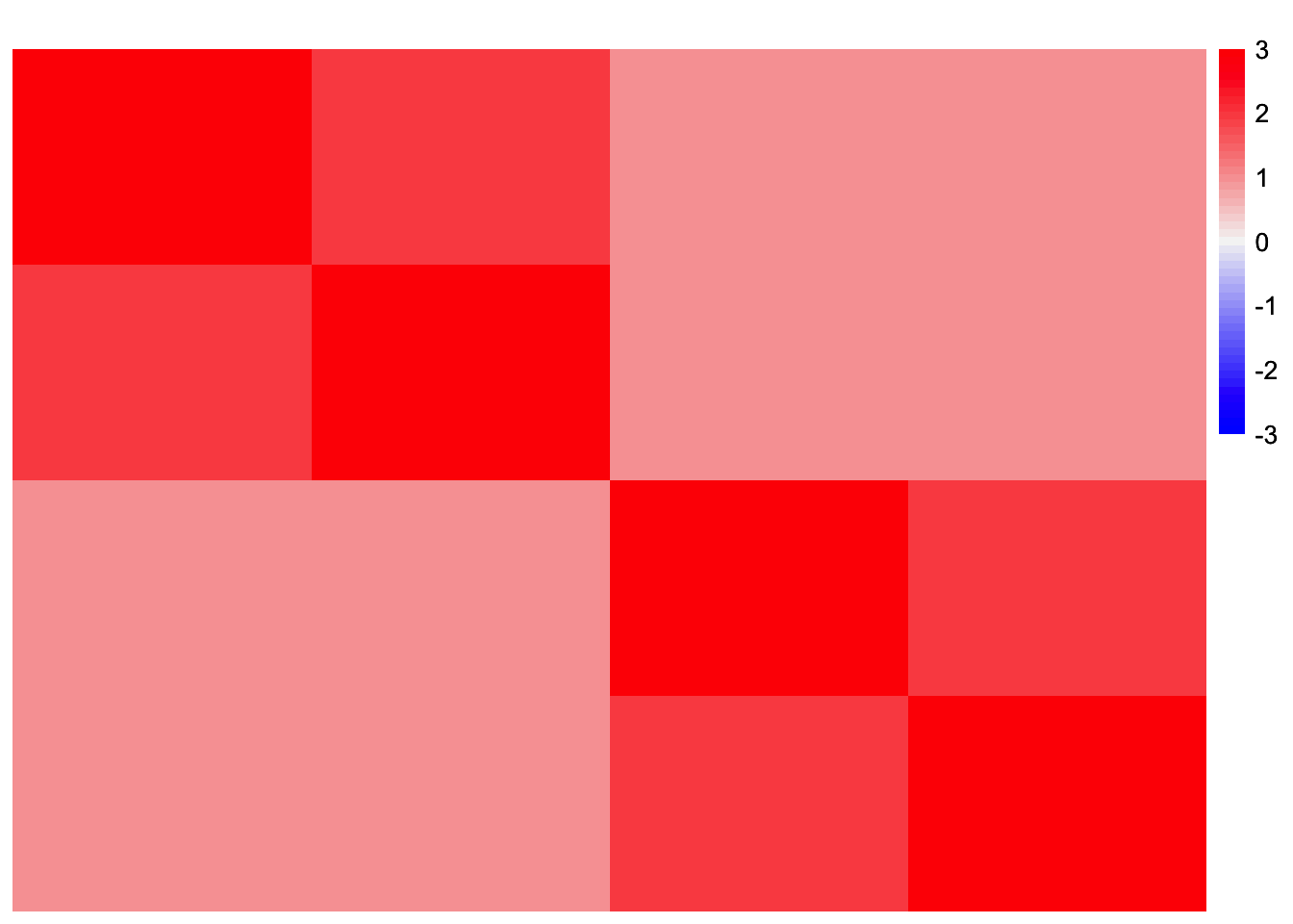
This is a plot of the first four eigenvectors:
YYt_orthog_no_noise_eigen <- eigen(YYt_orthog_no_noise)
plot_loadings(YYt_orthog_no_noise_eigen$vectors[,c(1:4)], bal_pops)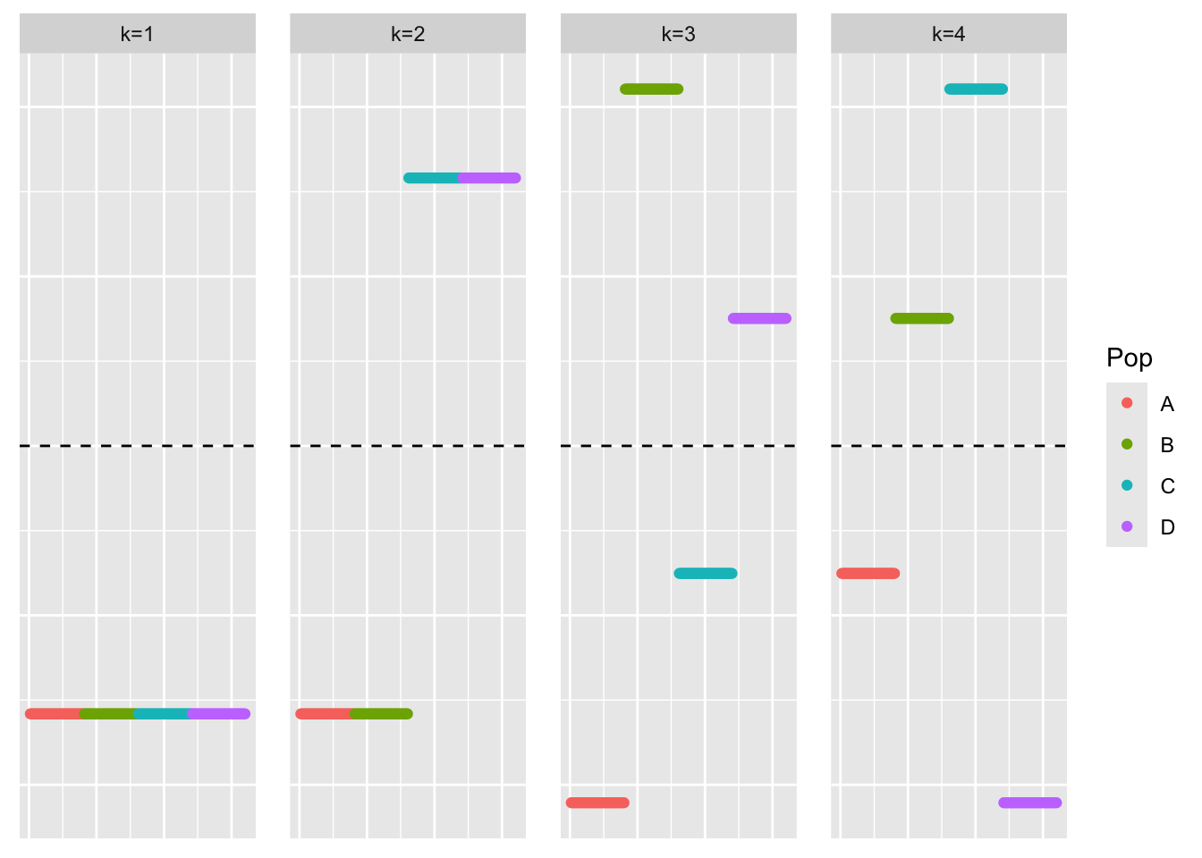
symebcovmf_no_noise_orthog_fit <- sym_ebcovmf_fit(S = YYt_orthog_no_noise, ebnm_fn = ebnm::ebnm_point_laplace, K = 4, maxiter = 500, rank_one_tol = 10^(-8), tol = 10^(-8), sign_constraint = NULL, refit_lam = TRUE)This is a plot of the loadings estimate, \(\hat{L}\):
plot_loadings(symebcovmf_no_noise_orthog_fit$L_pm, bal_pops)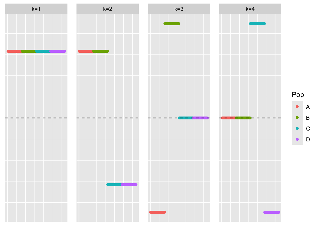
In this setting, the loadings estimate is the sparse representation. Perhaps \(F\) not being exactly orthogonal is why greedy-symEBcovMF is not finding the sparse representation?
Use orthogonal F in data generation
Now, I try generating noisy data with an orthogonal \(F\).
sim_args_orthog_F = list(pop_sizes = rep(40, 4), n_genes = 1000, branch_sds = rep(2,7), indiv_sd = 1, seed = 1, constrain_F = TRUE)
sim_data_orthog_F <- sim_4pops(sim_args_orthog_F)
This is a heatmap of the scaled Gram matrix:
plot_heatmap(sim_data_orthog_F$YYt, colors_range = c('blue','gray96','red'), brks = seq(-max(abs(sim_data_orthog_F$YYt)), max(abs(sim_data_orthog_F$YYt)), length.out = 50))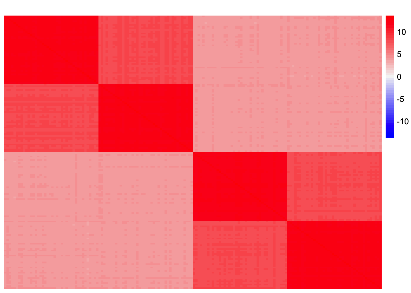
This is a scatter plot of the true loadings matrix:
pop_vec <- c(rep('A', 40), rep('B', 40), rep('C', 40), rep('D', 40))
plot_loadings(sim_data_orthog_F$LL, pop_vec)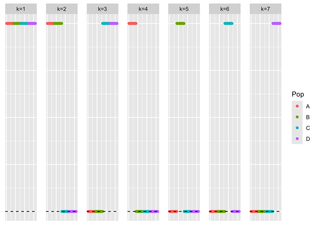
This is a plot of the eigenvalues of the Gram matrix:
S_orthog_F_eigen <- eigen(sim_data_orthog_F$YYt)
plot(S_orthog_F_eigen$values) + abline(a = 0, b = 0, col = 'red')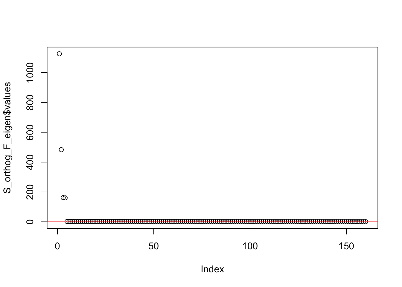
integer(0)This is the minimum eigenvalue:
min(S_orthog_F_eigen$values)[1] 0.3720117symEBcovMF
First, we start with running greedy symEBcovMF with the point-Laplace prior.
symebcovmf_orthog_F_fit <- sym_ebcovmf_fit(S = sim_data_orthog_F$YYt, ebnm_fn = ebnm::ebnm_point_laplace, K = 4, maxiter = 500, rank_one_tol = 10^(-8), tol = 10^(-8), sign_constraint = NULL, refit_lam = TRUE)This is a scatter plot of \(\hat{L}_{pt-laplace}\), the estimate from symEBcovMF:
bal_pops <- c(rep('A', 40), rep('B', 40), rep('C', 40), rep('D', 40))
plot_loadings(symebcovmf_orthog_F_fit$L_pm %*% diag(sqrt(symebcovmf_orthog_F_fit$lambda)), bal_pops)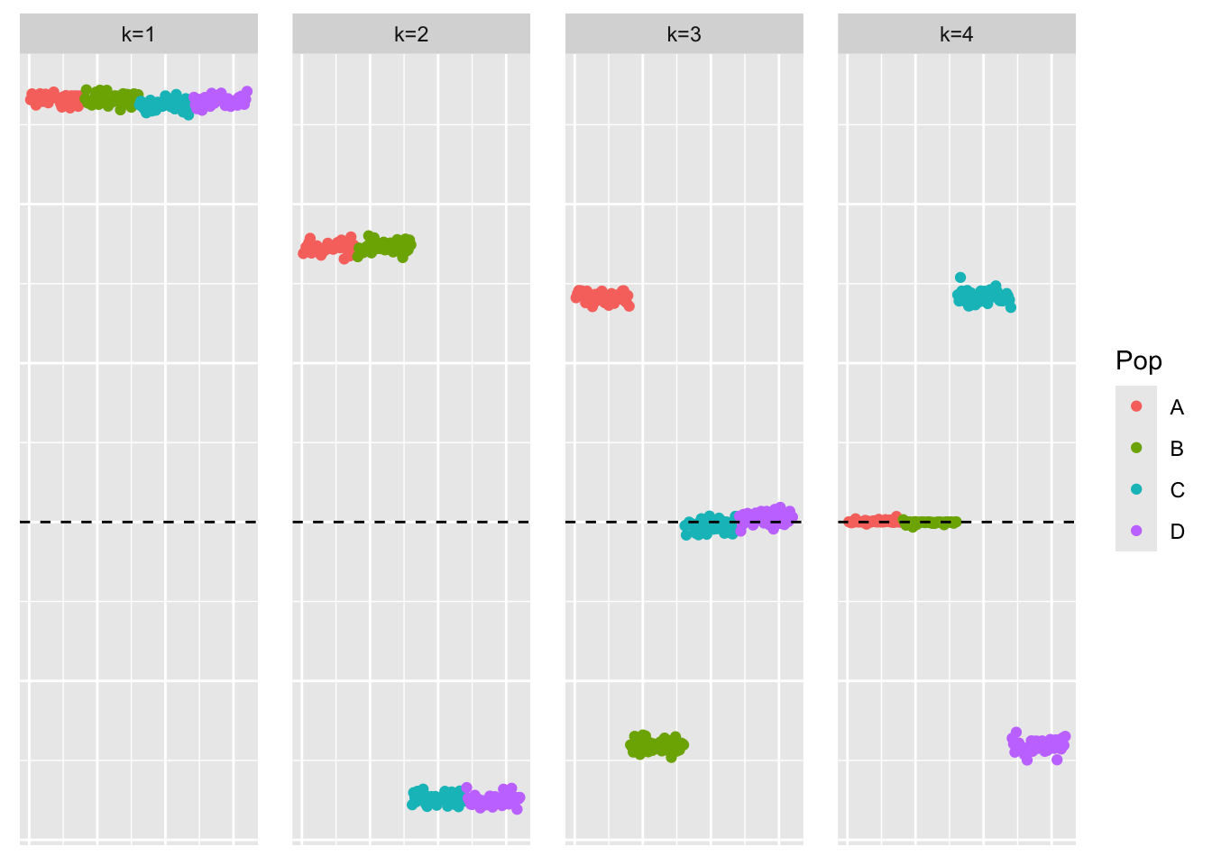
Observations
When we use an orthogonal \(F\) to generate the data, then greedy-symEBcovMF is able to find the sparse representation. This suggests that the method is influenced by the off-diagonal entries in \(S\) coming from correlations of the factors.
sessionInfo()R version 4.3.2 (2023-10-31)
Platform: aarch64-apple-darwin20 (64-bit)
Running under: macOS 15.4.1
Matrix products: default
BLAS: /Library/Frameworks/R.framework/Versions/4.3-arm64/Resources/lib/libRblas.0.dylib
LAPACK: /Library/Frameworks/R.framework/Versions/4.3-arm64/Resources/lib/libRlapack.dylib; LAPACK version 3.11.0
locale:
[1] en_US.UTF-8/en_US.UTF-8/en_US.UTF-8/C/en_US.UTF-8/en_US.UTF-8
time zone: America/New_York
tzcode source: internal
attached base packages:
[1] stats graphics grDevices utils datasets methods base
other attached packages:
[1] ggplot2_3.5.1 pheatmap_1.0.12 ebnm_1.1-34 workflowr_1.7.1
loaded via a namespace (and not attached):
[1] gtable_0.3.5 xfun_0.48 bslib_0.8.0 processx_3.8.4
[5] lattice_0.22-6 callr_3.7.6 vctrs_0.6.5 tools_4.3.2
[9] ps_1.7.7 generics_0.1.3 tibble_3.2.1 fansi_1.0.6
[13] highr_0.11 pkgconfig_2.0.3 Matrix_1.6-5 SQUAREM_2021.1
[17] RColorBrewer_1.1-3 lifecycle_1.0.4 truncnorm_1.0-9 farver_2.1.2
[21] compiler_4.3.2 stringr_1.5.1 git2r_0.33.0 munsell_0.5.1
[25] getPass_0.2-4 httpuv_1.6.15 htmltools_0.5.8.1 sass_0.4.9
[29] yaml_2.3.10 later_1.3.2 pillar_1.9.0 jquerylib_0.1.4
[33] whisker_0.4.1 cachem_1.1.0 trust_0.1-8 RSpectra_0.16-2
[37] tidyselect_1.2.1 digest_0.6.37 stringi_1.8.4 dplyr_1.1.4
[41] ashr_2.2-66 labeling_0.4.3 splines_4.3.2 rprojroot_2.0.4
[45] fastmap_1.2.0 grid_4.3.2 colorspace_2.1-1 cli_3.6.3
[49] invgamma_1.1 magrittr_2.0.3 utf8_1.2.4 withr_3.0.1
[53] scales_1.3.0 promises_1.3.0 horseshoe_0.2.0 rmarkdown_2.28
[57] httr_1.4.7 deconvolveR_1.2-1 evaluate_1.0.0 knitr_1.48
[61] irlba_2.3.5.1 rlang_1.1.4 Rcpp_1.0.13 mixsqp_0.3-54
[65] glue_1.8.0 rstudioapi_0.16.0 jsonlite_1.8.9 R6_2.5.1
[69] fs_1.6.4