symebcovmf_laplace_exploration
Annie Xie
2025-06-07
Last updated: 2025-06-19
Checks: 7 0
Knit directory:
symmetric_covariance_decomposition/
This reproducible R Markdown analysis was created with workflowr (version 1.7.1). The Checks tab describes the reproducibility checks that were applied when the results were created. The Past versions tab lists the development history.
Great! Since the R Markdown file has been committed to the Git repository, you know the exact version of the code that produced these results.
Great job! The global environment was empty. Objects defined in the global environment can affect the analysis in your R Markdown file in unknown ways. For reproduciblity it’s best to always run the code in an empty environment.
The command set.seed(20250408) was run prior to running
the code in the R Markdown file. Setting a seed ensures that any results
that rely on randomness, e.g. subsampling or permutations, are
reproducible.
Great job! Recording the operating system, R version, and package versions is critical for reproducibility.
Nice! There were no cached chunks for this analysis, so you can be confident that you successfully produced the results during this run.
Great job! Using relative paths to the files within your workflowr project makes it easier to run your code on other machines.
Great! You are using Git for version control. Tracking code development and connecting the code version to the results is critical for reproducibility.
The results in this page were generated with repository version 9d4fe22. See the Past versions tab to see a history of the changes made to the R Markdown and HTML files.
Note that you need to be careful to ensure that all relevant files for
the analysis have been committed to Git prior to generating the results
(you can use wflow_publish or
wflow_git_commit). workflowr only checks the R Markdown
file, but you know if there are other scripts or data files that it
depends on. Below is the status of the Git repository when the results
were generated:
Ignored files:
    Ignored:    .DS_Store
    Ignored:    .Rhistory

Untracked files:
    Untracked:  analysis/symebcovmf_point_exp_backfit_tree.Rmd
Note that any generated files, e.g. HTML, png, CSS, etc., are not included in this status report because it is ok for generated content to have uncommitted changes.
These are the previous versions of the repository in which changes were
made to the R Markdown
(analysis/symebcovmf_laplace_exploration.Rmd) and HTML
(docs/symebcovmf_laplace_exploration.html) files. If you’ve
configured a remote Git repository (see ?wflow_git_remote),
click on the hyperlinks in the table below to view the files as they
were in that past version.
| File | Version | Author | Date | Message |
|---|---|---|---|---|
| Rmd | 9d4fe22 | Annie Xie | 2025-06-19 | Update ELBO plot in laplace tree exploration |
| html | 2072809 | Annie Xie | 2025-06-13 | Build site. |
| Rmd | d3b42fa | Annie Xie | 2025-06-13 | Edit text in laplace exploration |
| html | 704e0a5 | Annie Xie | 2025-06-13 | Build site. |
| Rmd | 085c90f | Annie Xie | 2025-06-13 | Add exploration of point laplace in tree setting |
Introduction
In this analysis, we explore symEBcovMF with the point-Laplace prior in the tree setting.
Motivation
GBCD uses an initialization scheme that fits a point-Laplace prior fit. I wanted to try a similar initialization procedure for symEBcovMF. Therefore, I tried it on tree-structured data. When I tried it, I found that it didn’t work, and the reason it didn’t work is because the point-Laplace fit was not a divergence factorization. We expect that the symEBcovMF method should also be able to find a divergence factorization. Therefore, the purpose of this analysis is to explore why it does not.
Packages and Functions
library(ebnm)
library(pheatmap)
library(ggplot2)
source('code/visualization_functions.R')
source('code/symebcovmf_functions.R')compute_L2_fit <- function(est, dat){
score <- sum((dat - est)^2) - sum((diag(dat) - diag(est))^2)
return(score)
}Backfit Functions
optimize_factor <- function(R, ebnm_fn, maxiter, tol, v_init, lambda_k, R2k, n, KL){
  R2 <- R2k - lambda_k^2
  resid_s2 <- estimate_resid_s2(n = n, R2 = R2)
  rank_one_KL <- 0
  curr_elbo <- -Inf
  obj_diff <- Inf
  fitted_g_k <- NULL
  iter <- 1
  vec_elbo_full <- NULL
  v <- v_init

  while((iter <= maxiter) && (obj_diff > tol)){
    # update l; power iteration step
    v.old <- v
    x <- R %*% v
    e <- ebnm_fn(x = x, s = sqrt(resid_s2), g_init = fitted_g_k)
    scaling_factor <- sqrt(sum(e$posterior$mean^2) + sum(e$posterior$sd^2))
    if (scaling_factor == 0){ # check if scaling factor is zero
      scaling_factor <- Inf
      v <- e$posterior$mean/scaling_factor
      print('Warning: scaling factor is zero')
      break
    }
    v <- e$posterior$mean/scaling_factor

    # update lambda and R2
    lambda_k.old <- lambda_k
    lambda_k <- max(as.numeric(t(v) %*% R %*% v), 0)
    R2 <- R2k - lambda_k^2

    #store estimate for g
    fitted_g_k.old <- fitted_g_k
    fitted_g_k <- e$fitted_g

    # store KL
    rank_one_KL.old <- rank_one_KL
    rank_one_KL <- as.numeric(e$log_likelihood) +
      - normal_means_loglik(x, sqrt(resid_s2), e$posterior$mean, e$posterior$mean^2 + e$posterior$sd^2)

    # update resid_s2
    resid_s2.old <- resid_s2
    resid_s2 <- estimate_resid_s2(n = n, R2 = R2) # this goes negative?????

    # check convergence - maybe change to rank-one obj function
    curr_elbo.old <- curr_elbo
    curr_elbo <- compute_elbo(resid_s2 = resid_s2,
                              n = n,
                              KL = c(KL, rank_one_KL),
                              R2 = R2)
    if (iter > 1){
      obj_diff <- curr_elbo - curr_elbo.old
    }
    if (obj_diff < 0){ # check if convergence_val < 0
      v <- v.old
      resid_s2 <- resid_s2.old
      rank_one_KL <- rank_one_KL.old
      lambda_k <- lambda_k.old
      curr_elbo <- curr_elbo.old
      fitted_g_k <- fitted_g_k.old
      print(paste('elbo decreased by', abs(obj_diff)))
      break
    }
    vec_elbo_full <- c(vec_elbo_full, curr_elbo)
    iter <- iter + 1
  }
  return(list(v = v, lambda_k = lambda_k, resid_s2 = resid_s2, curr_elbo = curr_elbo, vec_elbo_full = vec_elbo_full, fitted_g_k = fitted_g_k, rank_one_KL = rank_one_KL))
}
#nullcheck function
nullcheck_factors <- function(sym_ebcovmf_obj, L2_tol = 10^(-8)){
null_lambda_idx <- which(sym_ebcovmf_obj$lambda == 0)
factor_L2_norms <- apply(sym_ebcovmf_obj$L_pm, 2, function(v){sqrt(sum(v^2))})
null_factor_idx <- which(factor_L2_norms < L2_tol)
null_idx <- unique(c(null_lambda_idx, null_factor_idx))
keep_idx <- setdiff(c(1:length(sym_ebcovmf_obj$lambda)), null_idx)
if (length(keep_idx) < length(sym_ebcovmf_obj$lambda)){
#remove factors
sym_ebcovmf_obj$L_pm <- sym_ebcovmf_obj$L_pm[,keep_idx]
sym_ebcovmf_obj$lambda <- sym_ebcovmf_obj$lambda[keep_idx]
sym_ebcovmf_obj$KL <- sym_ebcovmf_obj$KL[keep_idx]
sym_ebcovmf_obj$fitted_gs <- sym_ebcovmf_obj$fitted_gs[keep_idx]
}
#shouldn't need to recompute objective function or other things
return(sym_ebcovmf_obj)
}sym_ebcovmf_backfit <- function(S, sym_ebcovmf_obj, ebnm_fn, backfit_maxiter = 100, backfit_tol = 10^(-8), optim_maxiter= 500, optim_tol = 10^(-8)){
K <- length(sym_ebcovmf_obj$lambda)
iter <- 1
obj_diff <- Inf
sym_ebcovmf_obj$backfit_vec_elbo_full <- NULL
sym_ebcovmf_obj$backfit_iter_elbo_vec <- NULL
# refit lambda
sym_ebcovmf_obj <- refit_lambda(S, sym_ebcovmf_obj, maxiter = 25)
while((iter <= backfit_maxiter) && (obj_diff > backfit_tol)){
# print(iter)
obj_old <- sym_ebcovmf_obj$elbo
# loop through each factor
for (k in 1:K){
# print(k)
# compute residual matrix
R <- S - tcrossprod(sym_ebcovmf_obj$L_pm[,-k] %*% diag(sqrt(sym_ebcovmf_obj$lambda[-k]), ncol = (K-1)))
R2k <- compute_R2(S, sym_ebcovmf_obj$L_pm[,-k], sym_ebcovmf_obj$lambda[-k], (K-1)) #this is right but I have one instance where the values don't match what I expect
# optimize factor
factor_proposed <- optimize_factor(R, ebnm_fn, optim_maxiter, optim_tol, sym_ebcovmf_obj$L_pm[,k], sym_ebcovmf_obj$lambda[k], R2k, sym_ebcovmf_obj$n, sym_ebcovmf_obj$KL[-k])
# update object
sym_ebcovmf_obj$L_pm[,k] <- factor_proposed$v
sym_ebcovmf_obj$KL[k] <- factor_proposed$rank_one_KL
sym_ebcovmf_obj$lambda[k] <- factor_proposed$lambda_k
sym_ebcovmf_obj$resid_s2 <- factor_proposed$resid_s2
sym_ebcovmf_obj$fitted_gs[[k]] <- factor_proposed$fitted_g_k
sym_ebcovmf_obj$elbo <- factor_proposed$curr_elbo
sym_ebcovmf_obj$backfit_vec_elbo_full <- c(sym_ebcovmf_obj$backfit_vec_elbo_full, factor_proposed$vec_elbo_full)
#print(sym_ebcovmf_obj$elbo)
sym_ebcovmf_obj <- refit_lambda(S, sym_ebcovmf_obj) # add refitting step?
#print(sym_ebcovmf_obj$elbo)
}
sym_ebcovmf_obj$backfit_iter_elbo_vec <- c(sym_ebcovmf_obj$backfit_iter_elbo_vec, sym_ebcovmf_obj$elbo)
iter <- iter + 1
obj_diff <- abs(sym_ebcovmf_obj$elbo - obj_old)
# need to add check if it is negative?
}
# nullcheck
sym_ebcovmf_obj <- nullcheck_factors(sym_ebcovmf_obj)
return(sym_ebcovmf_obj)
}Data Generation
To test this procedure, I will apply it to the tree-structured dataset.
sim_4pops <- function(args) {
  set.seed(args$seed)

  n <- sum(args$pop_sizes)
  p <- args$n_genes

  FF <- matrix(rnorm(7 * p, sd = rep(args$branch_sds, each = p)), ncol = 7)
  # if (args$constrain_F) {
  #   FF_svd <- svd(FF)
  #   FF <- FF_svd$u
  #   FF <- t(t(FF) * branch_sds * sqrt(p))
  # }

  LL <- matrix(0, nrow = n, ncol = 7)
  LL[, 1] <- 1
  LL[, 2] <- rep(c(1, 1, 0, 0), times = args$pop_sizes)
  LL[, 3] <- rep(c(0, 0, 1, 1), times = args$pop_sizes)
  LL[, 4] <- rep(c(1, 0, 0, 0), times = args$pop_sizes)
  LL[, 5] <- rep(c(0, 1, 0, 0), times = args$pop_sizes)
  LL[, 6] <- rep(c(0, 0, 1, 0), times = args$pop_sizes)
  LL[, 7] <- rep(c(0, 0, 0, 1), times = args$pop_sizes)

  E <- matrix(rnorm(n * p, sd = args$indiv_sd), nrow = n)
  Y <- LL %*% t(FF) + E
  YYt <- (1/p)*tcrossprod(Y)
  return(list(Y = Y, YYt = YYt, LL = LL, FF = FF, K = ncol(LL)))
}
sim_args = list(pop_sizes = rep(40, 4), n_genes = 1000, branch_sds = rep(2,7), indiv_sd = 1, seed = 1)
sim_data <- sim_4pops(sim_args)This is a heatmap of the scaled Gram matrix:
plot_heatmap(sim_data$YYt, colors_range = c('blue','gray96','red'), brks = seq(-max(abs(sim_data$YYt)), max(abs(sim_data$YYt)), length.out = 50))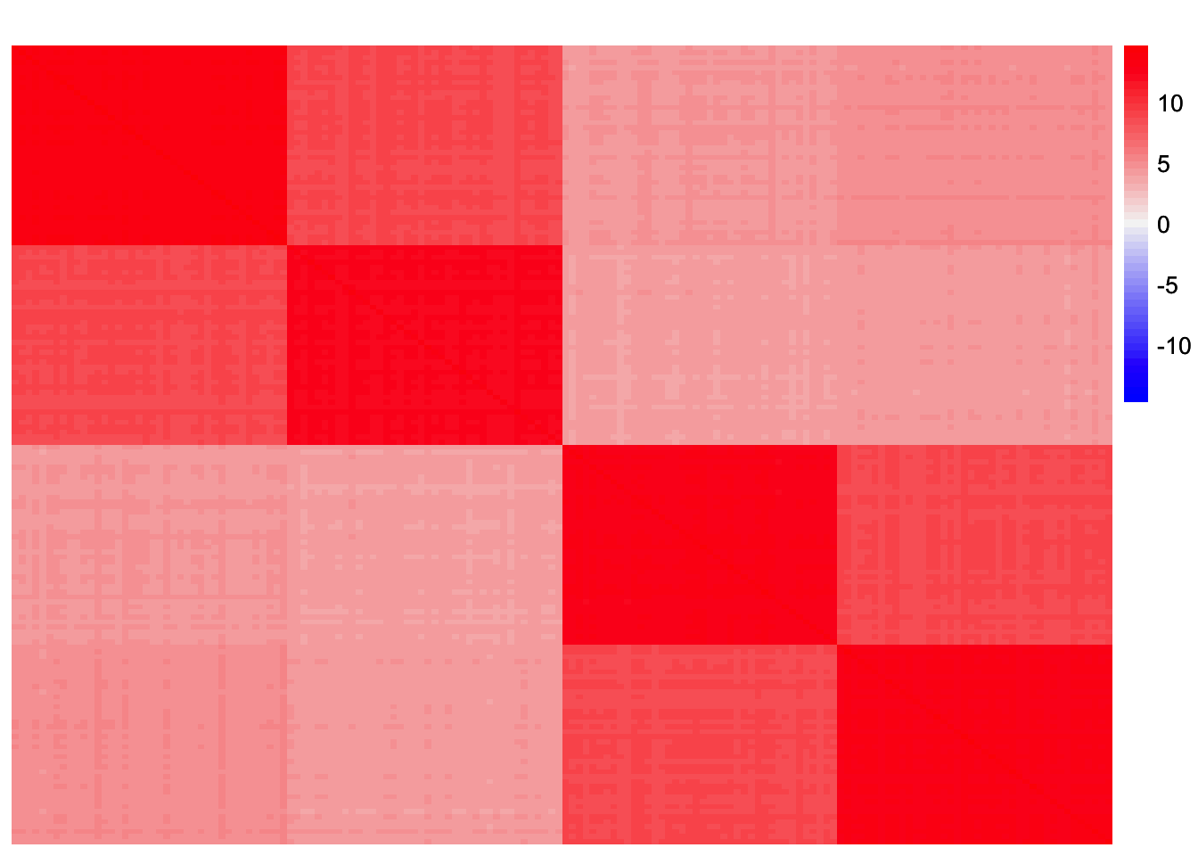
| Version | Author | Date |
|---|---|---|
| 704e0a5 | Annie Xie | 2025-06-13 |
This is a scatter plot of the true loadings matrix:
pop_vec <- c(rep('A', 40), rep('B', 40), rep('C', 40), rep('D', 40))
plot_loadings(sim_data$LL, pop_vec)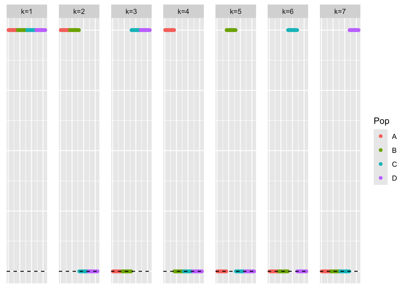
| Version | Author | Date |
|---|---|---|
| 704e0a5 | Annie Xie | 2025-06-13 |
This is a plot of the eigenvalues of the Gram matrix:
S_eigen <- eigen(sim_data$YYt)
plot(S_eigen$values) + abline(a = 0, b = 0, col = 'red')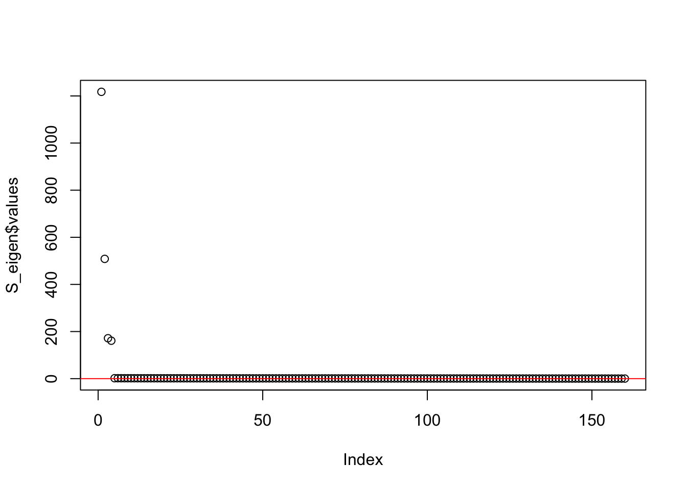
| Version | Author | Date |
|---|---|---|
| 704e0a5 | Annie Xie | 2025-06-13 |
integer(0)This is the minimum eigenvalue:
min(S_eigen$values)[1] 0.3724341symEBcovMF with point-Laplace
First, we start with running greedy symEBcovMF with the point-Laplace prior.
symebcovmf_fit <- sym_ebcovmf_fit(S = sim_data$YYt, ebnm_fn = ebnm::ebnm_point_laplace, K = 7, maxiter = 500, rank_one_tol = 10^(-8), tol = 10^(-8), sign_constraint = NULL, refit_lam = TRUE)[1] "Warning: scaling factor is zero"
[1] "Adding factor 5 does not improve the objective function"This is a scatter plot of \(\hat{L}_{pt-laplace}\), the estimate from symEBcovMF:
bal_pops <- c(rep('A', 40), rep('B', 40), rep('C', 40), rep('D', 40))
plot_loadings(symebcovmf_fit$L_pm %*% diag(sqrt(symebcovmf_fit$lambda)), bal_pops)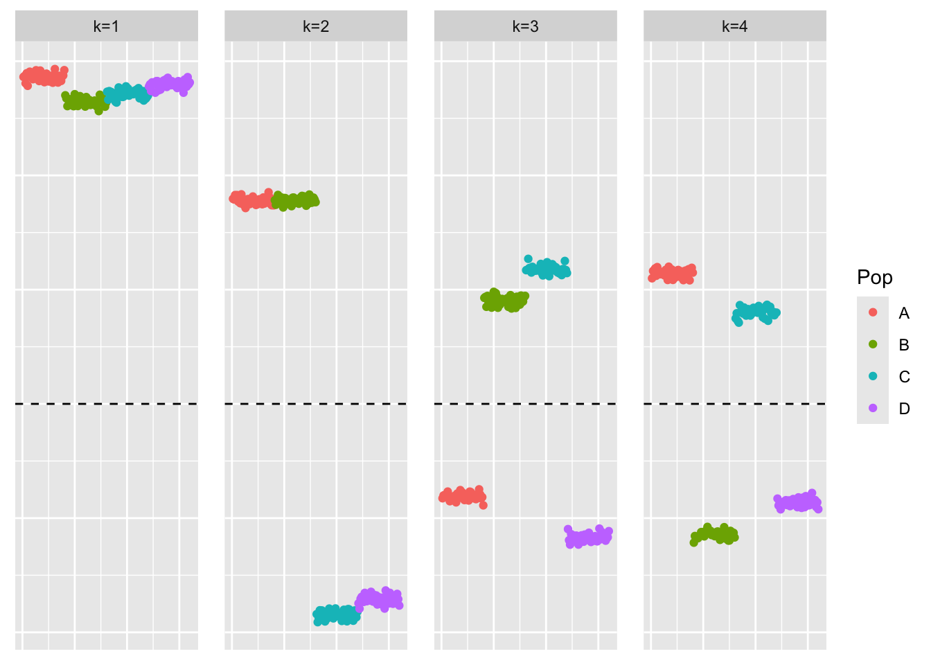
| Version | Author | Date |
|---|---|---|
| 704e0a5 | Annie Xie | 2025-06-13 |
This is the objective function value attained:
symebcovmf_fit$elbo[1] -10362.6Observations
symEBcovMF with point-Laplace prior does not find a divergence factorization. We want the third factor to have zero loading for one branch of populations, and then positive loading for one population and negative loading for the remaining population. We want something analogous for the fourth factor. However, symEBcovMF has found a different third and fourth factor.
Intuitively, the sparser representation should have a higher objective function value due to the sparsity-inducing prior. So we would expect the method to find the sparser representation.
Additional Backfit
GBCD does additional backfitting on the point-Laplace fit, so here I test how additional backfitting performs. However, Matthew told me that he thinks it would be difficult to recover the sparse representation from the backfit since all the factors are non-sparse and reinforce each other. In this analysis, I run the backfitting for more iterations than in the original analysis.
This is the code for the backfit:
symebcovmf_fit_backfit <- sym_ebcovmf_backfit(sim_data$YYt, symebcovmf_fit, ebnm_fn = ebnm_point_laplace, backfit_maxiter = 20000)I will load in previously saved results:
symebcovmf_fit_backfit <- readRDS('data/symebcovmf_laplace_tree_backfit_20000.rds')This is a scatter plot of \(\hat{L}_{pt-laplace-backfit}\), the estimate from symEBcovMF with backfit:
bal_pops <- c(rep('A', 40), rep('B', 40), rep('C', 40), rep('D', 40))
plot_loadings(symebcovmf_fit_backfit$L_pm %*% diag(sqrt(symebcovmf_fit_backfit$lambda)), bal_pops)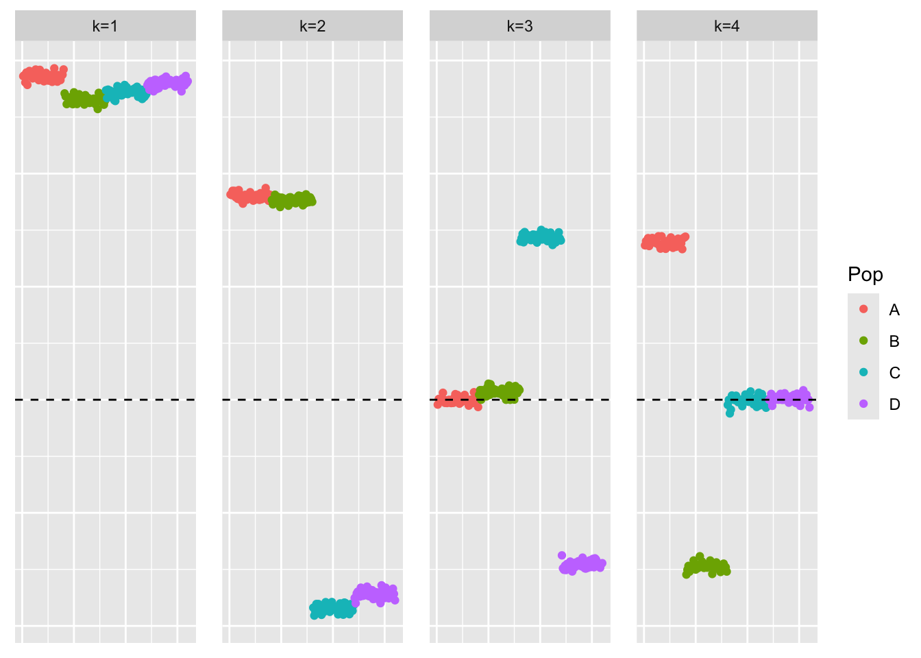
This is the objective function value attained:
symebcovmf_fit_backfit$elbo[1] 9576.714This is a plot of the progression of the ELBO:
plot(symebcovmf_fit_backfit$backfit_iter_elbo_vec, ylab = 'ELBO')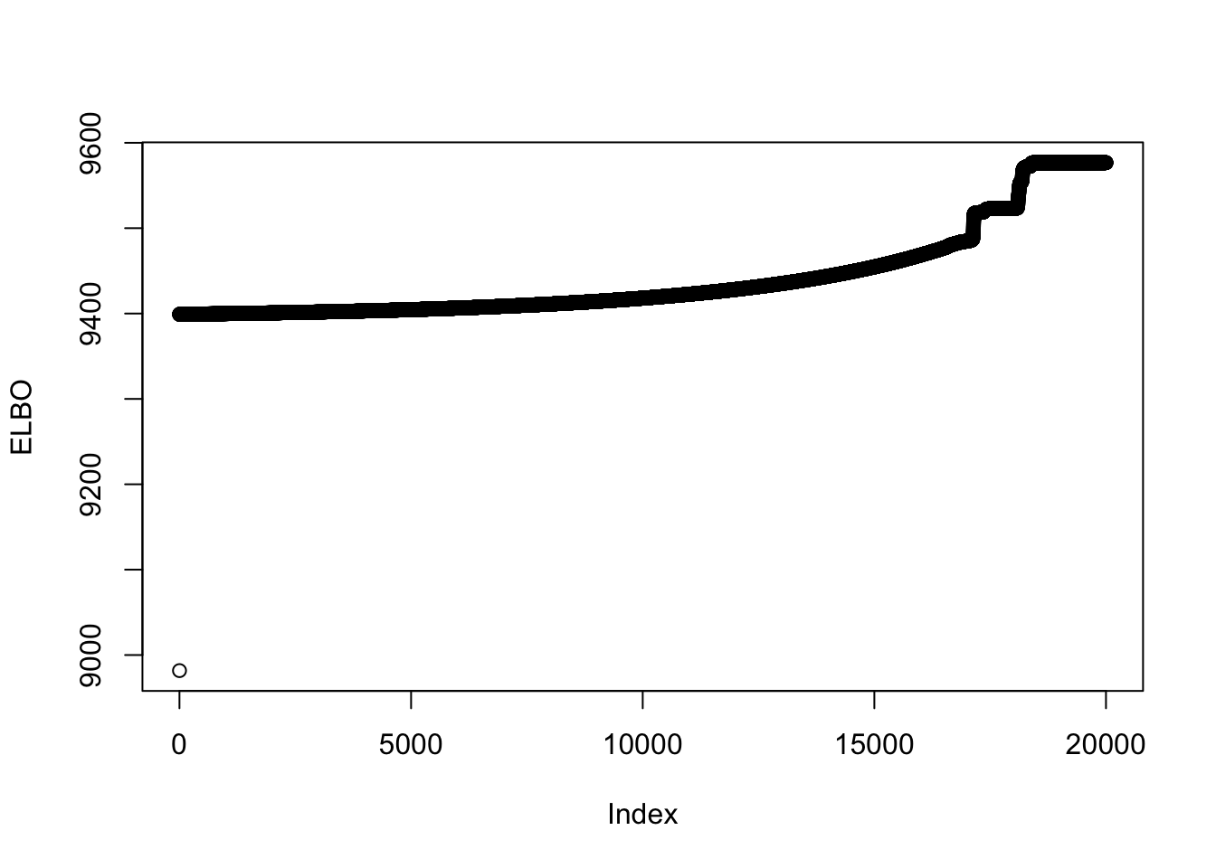
These plots are a closer look at the progression of the ELBO:
plot(x = c(1:5000), y = symebcovmf_fit_backfit$backfit_iter_elbo_vec[1:5000], xlab = 'Index', ylab = 'ELBO', main = 'ELBO for Iterations 1-5000')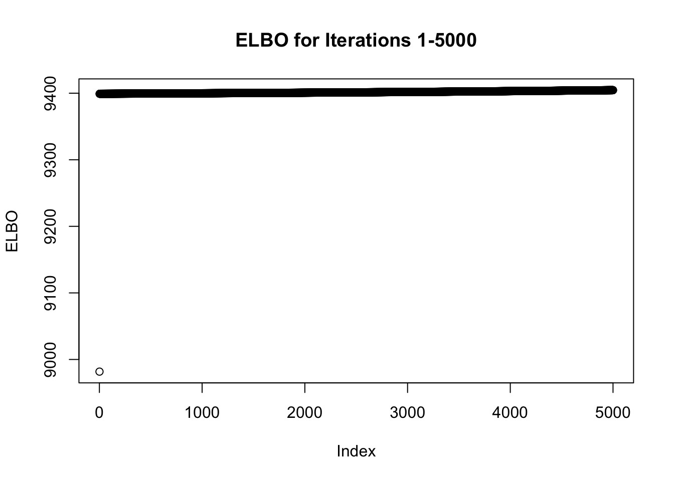
plot(x = c(5000:10000), y = symebcovmf_fit_backfit$backfit_iter_elbo_vec[5000:10000], xlab = 'Index', ylab = 'ELBO', main = 'ELBO for Iterations 5000-10000')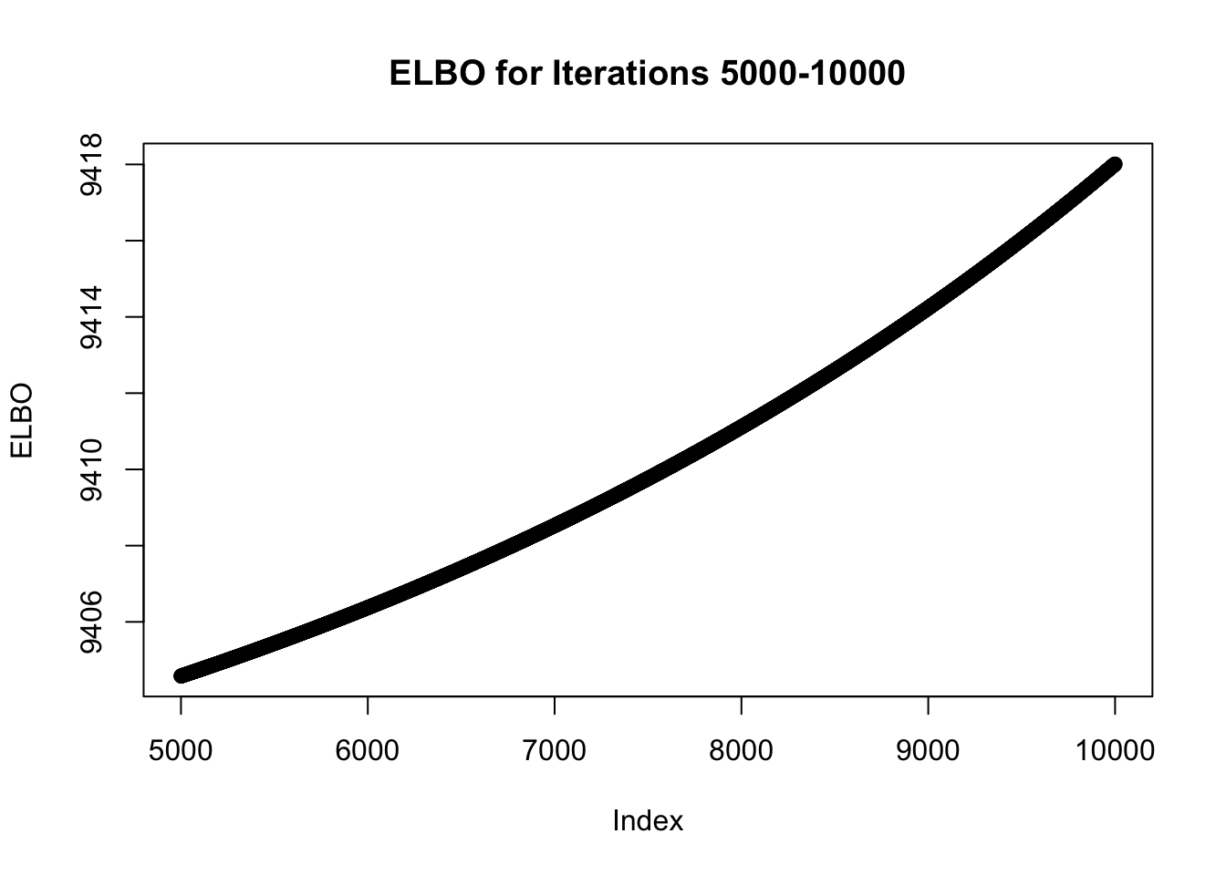
| Version | Author | Date |
|---|---|---|
| 704e0a5 | Annie Xie | 2025-06-13 |
plot(x = c(10000:15000), y = symebcovmf_fit_backfit$backfit_iter_elbo_vec[10000:15000], xlab = 'Index', ylab = 'ELBO', main = 'ELBO for Iterations 10000-15000')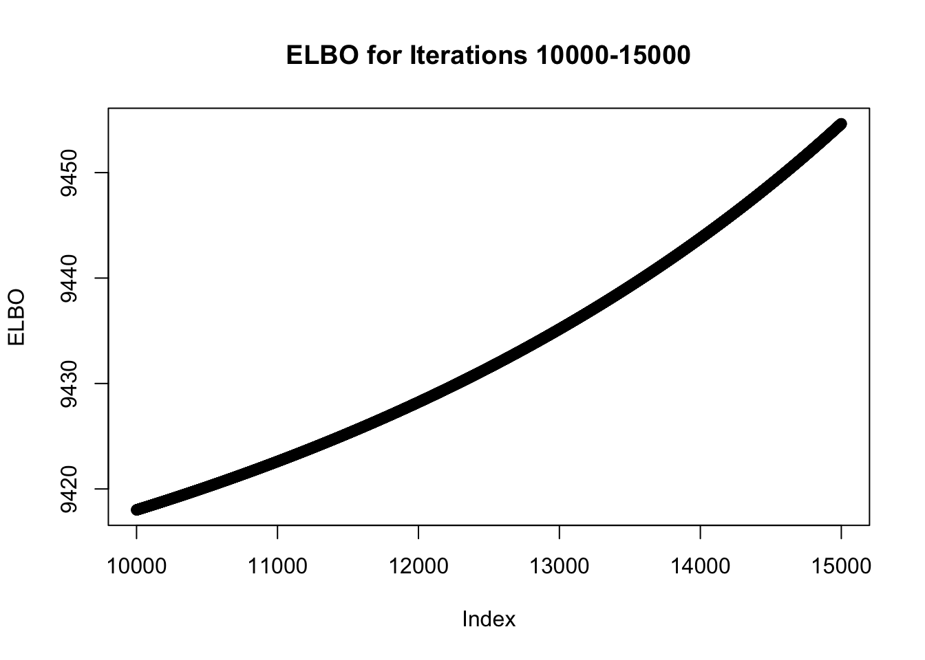
| Version | Author | Date |
|---|---|---|
| 704e0a5 | Annie Xie | 2025-06-13 |
plot(x = c(15000:20000), y = symebcovmf_fit_backfit$backfit_iter_elbo_vec[15000:20000], xlab = 'Index', ylab = 'ELBO', main = 'ELBO for Iterations 15000-20000')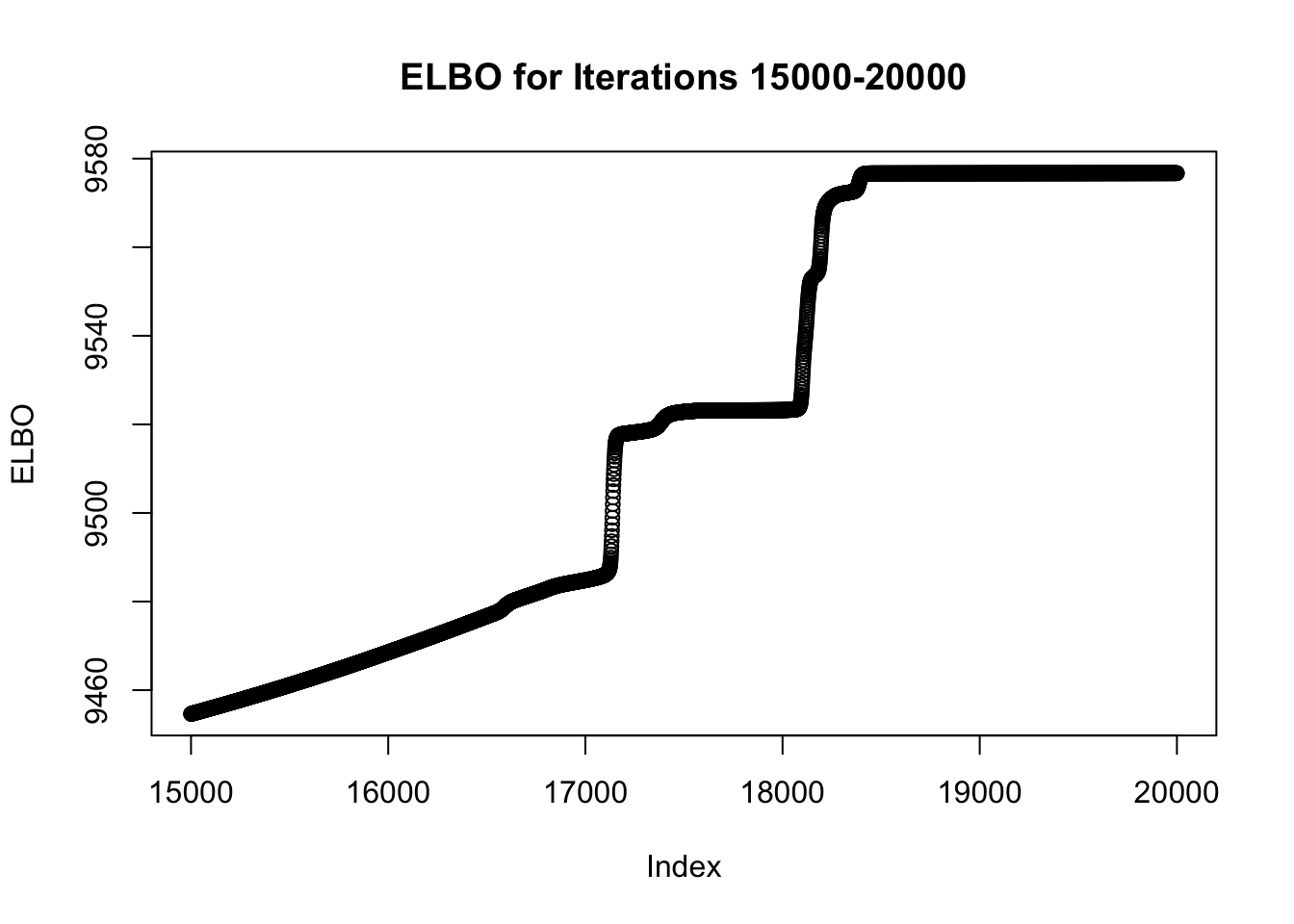
I tested backfitting for various numbers of iterations. If I backfit for longer, e.g. at least 20,000 iterations, then eventually the method finds the sparse representation. Therefore, the method does work when backfit for long enough.
Exploration of other methods
I want to compare the performance of symEBcovMF to that of other methods, in particular flashier and EBCD.
Flashier
First, we run greedy-flash on \(S\):
library(flashier)flash_cov_fit <- flash_init(data = sim_data$YYt) |>
flash_greedy(Kmax = 4, ebnm_fn = ebnm::ebnm_point_laplace)Adding factor 1 to flash object...
Adding factor 2 to flash object...
Adding factor 3 to flash object...
Adding factor 4 to flash object...
Wrapping up...
Done.This is a plot of the loadings estimate, \(\hat{L}_{flash}\):
plot_loadings(flash_cov_fit$L_pm, bal_pops)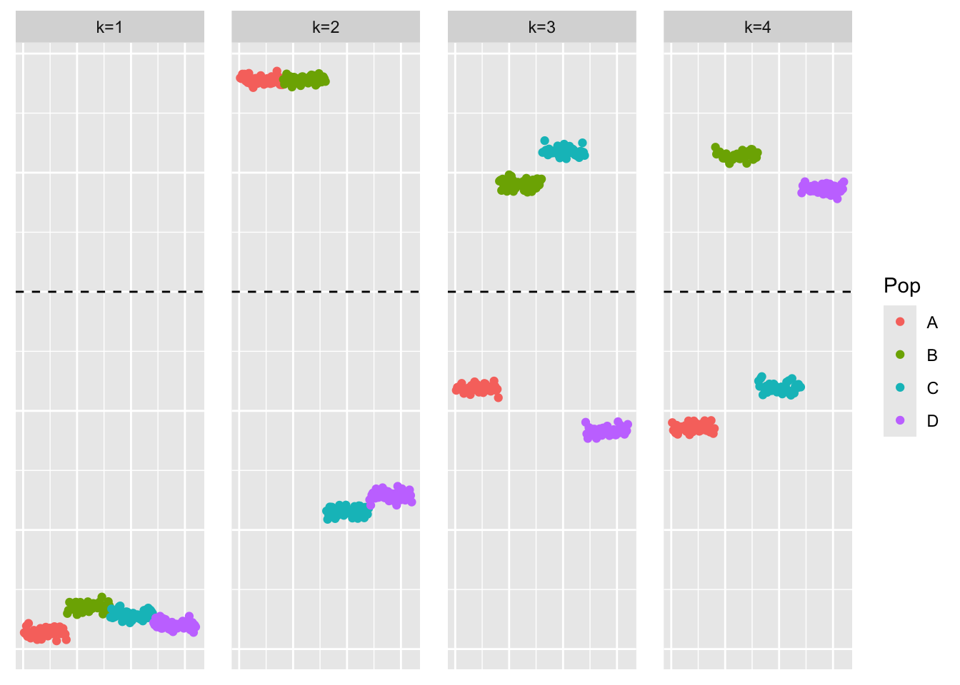
This is a plot of the factor estimate, \(\hat{F}_{flash}\). Note that because \(S\) is symmetric, we expect the loadings estimate and factor estimate to be about the same (up to a scaling):
plot_loadings(flash_cov_fit$F_pm, bal_pops)
We see that the loadings estimate looks similar to what greedy-symEBcovMF found.
Now, we try backfitting.
flash_cov_backfit_fit <- flash_cov_fit |>
  flash_backfit(maxiter = 100)
Backfitting 4 factors (tolerance: 3.81e-04)...
Difference between iterations is within 1.0e+04...
Difference between iterations is within 1.0e+03...
Difference between iterations is within 1.0e+02...
Difference between iterations is within 1.0e+01...
Difference between iterations is within 1.0e+00...
Difference between iterations is within 1.0e-01...
Difference between iterations is within 1.0e-02...
Difference between iterations is within 1.0e-03...
Wrapping up...
Done.This is a plot of the loadings estimate, \(\hat{L}_{flash-backfit}\):
plot_loadings(flash_cov_backfit_fit$L_pm, bal_pops)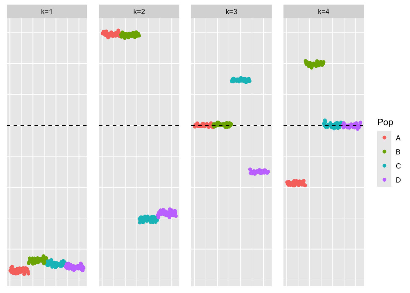
| Version | Author | Date |
|---|---|---|
| 704e0a5 | Annie Xie | 2025-06-13 |
This is a plot of the factor estimate, \(\hat{F}_{flash-backfit}\).
plot_loadings(flash_cov_backfit_fit$F_pm, bal_pops)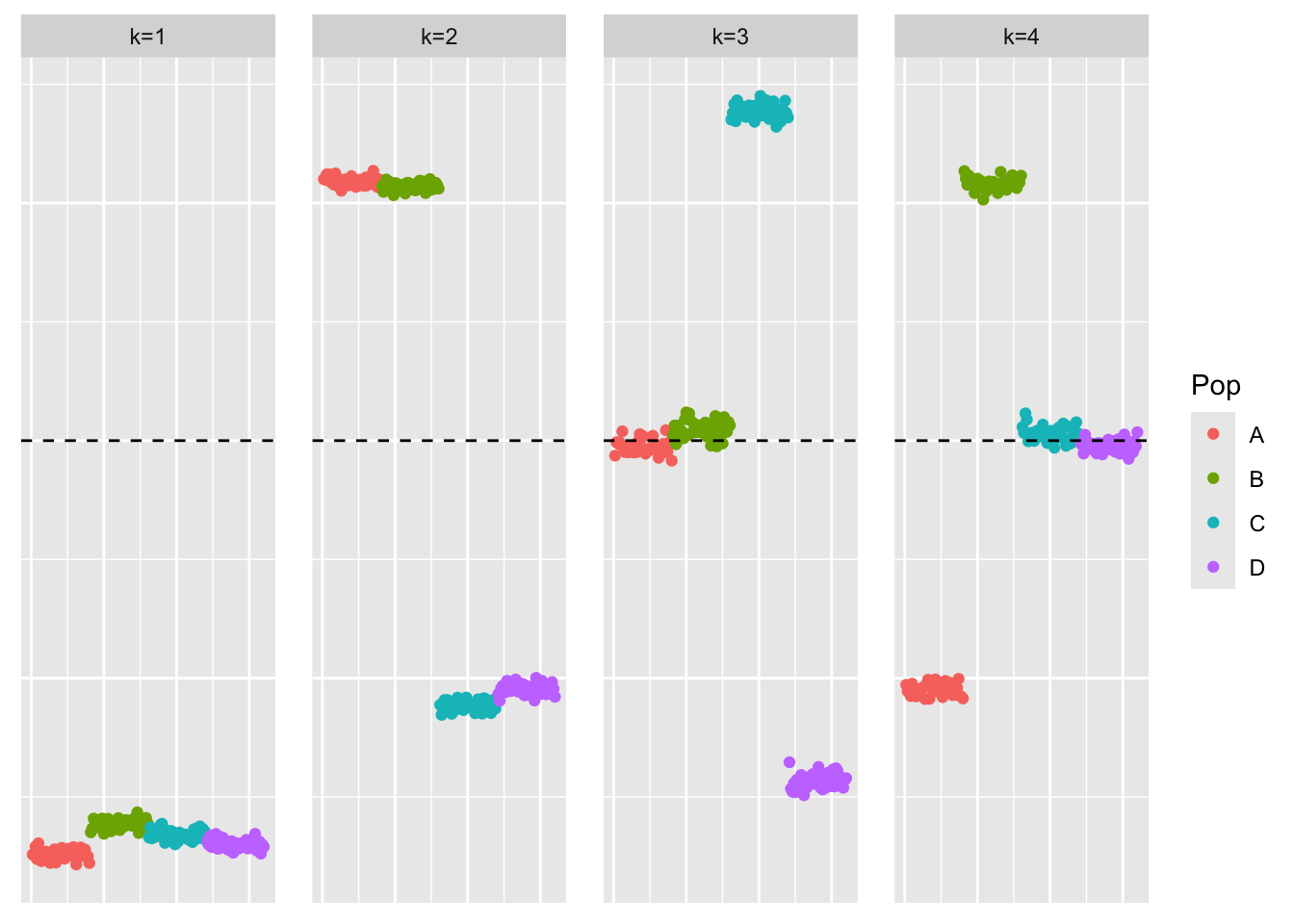
When applying greedy-flash to the Gram matrix, we get a similar estimate to that of greedy symEBcovMF. In particular, the third and fourth factors are not sparse. However, after backfitting, the method finds the sparse representation. Flashier only requires about 100 backfit iterations to yield an estimate which looks sparse. The backfit procedure for flashier seems to be much faster than the backfit procedure for symEBcovMF. I’m not sure if this is due to coding or the choice of convergence tolerance or something else. I imagine that EBMFcov has a similar performance to flashier.
EBMFcov
We also test EBMFcov. First, we try the version of EBMFcov that fits the flashier fit with the greedy method.
cov_fit <- function(covmat, ebnm_fn = ebnm::ebnm_point_laplace, Kmax = 1000, verbose.lvl = 0, backfit = FALSE, backfit_maxiter = 500) {
  fl <- flash_init(covmat, var_type = 0) |>
    flash_set_verbose(verbose.lvl) |>
    flash_greedy(ebnm_fn = ebnm_fn, Kmax = Kmax)
  if (backfit == TRUE){
      fl <- fl |>
        flash_backfit(maxiter = backfit_maxiter)
    }
  s2 <- max(0, mean(diag(covmat) - diag(fitted(fl))))
  s2_diff <- Inf
  while(s2 > 0 && abs(s2_diff - 1) > 1e-4) {
    covmat_minuss2 <- covmat - diag(rep(s2, ncol(covmat)))
    fl <- fl |>
      flash_update_data(covmat_minuss2) |>
      flash_set_verbose(verbose.lvl)
    if (backfit == TRUE){
      fl <- fl |>
        flash_backfit(maxiter = backfit_maxiter)
    }
    old_s2 <- s2
    s2 <- max(0, mean(diag(covmat) - diag(fitted(fl))))
    s2_diff <- s2 / old_s2
  }

  return(list(fl=fl, s2 = s2))
}
ebmfcov_diag_fit <- cov_fit(sim_data$YYt,
ebnm::ebnm_point_laplace,
Kmax = 4)This is a plot of the loadings estimate, \(\hat{L}_{ebmfcov}\):
plot_loadings(ebmfcov_diag_fit$fl$L_pm, bal_pops)
This is a plot of the factor estimate, \(\hat{F}_{ebmfcov}\). Note that because \(S\) is symmetric, we expect the loadings estimate and factor estimate to be about the same (up to a scaling):
plot_loadings(ebmfcov_diag_fit$fl$F_pm, bal_pops)
Similar to flash, the loadings estimate looks similar to what greedy-symEBcovMF found.
Now, we try adding backfitting.
ebmfcov_diag_backfit_fit <- cov_fit(sim_data$YYt,
                             ebnm::ebnm_point_laplace,
                             Kmax = 4, backfit = TRUE)
This is a plot of the loadings estimate, \(\hat{L}_{ebmfcov-backfit}\):
plot_loadings(ebmfcov_diag_backfit_fit$fl$L_pm, bal_pops)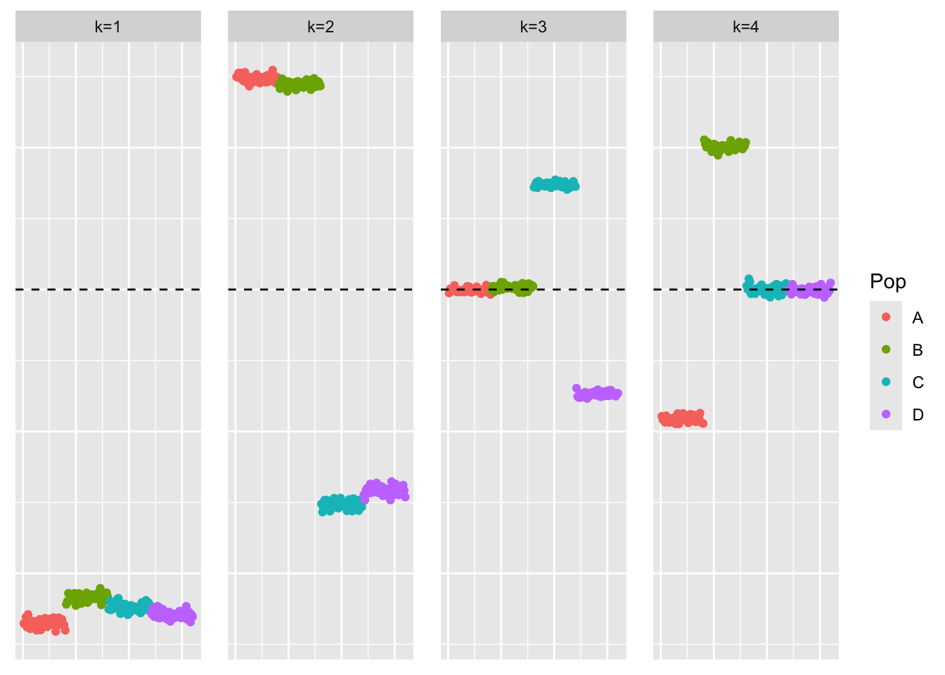
This is a plot of the factor estimate, \(\hat{F}_{ebmfcov-backfit}\).
plot_loadings(ebmfcov_diag_backfit_fit$fl$F_pm, bal_pops)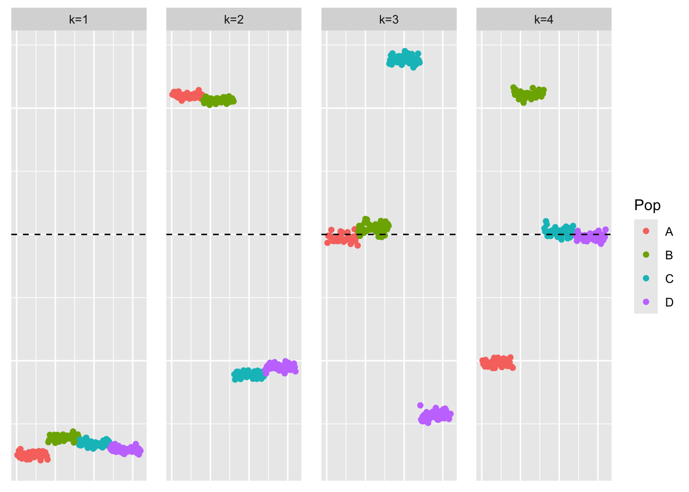
| Version | Author | Date |
|---|---|---|
| 704e0a5 | Annie Xie | 2025-06-13 |
When we add backfitting to the procedure, we see that the method does find the sparse representation.
EBCD
We also test EBCD. First, we apply EBCD’s greedy initialization procedure.
library(ebcd)set.seed(1)
ebcd_init_obj <- ebcd_init(X = t(sim_data$Y))
ebcd_greedy_fit <- ebcd_greedy(ebcd_init_obj, Kmax = 4, ebnm_fn = ebnm::ebnm_point_laplace)This is a plot of the loadings estimate \(\hat{L}_{ebcd-greedy}\):
plot_loadings(ebcd_greedy_fit$EL, bal_pops)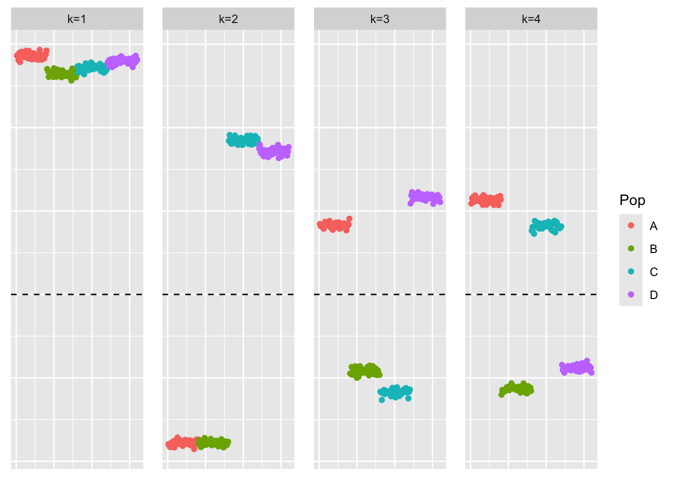
Now, we backfit.
ebcd_fit <- ebcd_backfit(ebcd_greedy_fit)This is a plot of the loadings estimate \(\hat{L}_{ebcd-backfit}\):
plot_loadings(ebcd_fit$EL, bal_pops)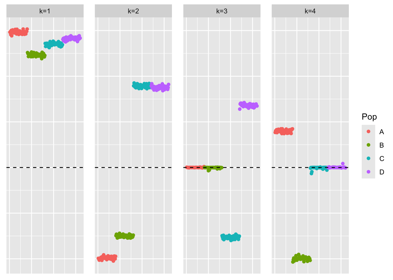
For EBCD, we see similar performance – the greedy method finds a representation that is not sparse, and the backfitting yields the sparse representation. Question: is the backfit of the these methods faster than that of symEBcovMF?
sessionInfo()R version 4.3.2 (2023-10-31)
Platform: aarch64-apple-darwin20 (64-bit)
Running under: macOS 15.4.1
Matrix products: default
BLAS: /Library/Frameworks/R.framework/Versions/4.3-arm64/Resources/lib/libRblas.0.dylib
LAPACK: /Library/Frameworks/R.framework/Versions/4.3-arm64/Resources/lib/libRlapack.dylib; LAPACK version 3.11.0
locale:
[1] en_US.UTF-8/en_US.UTF-8/en_US.UTF-8/C/en_US.UTF-8/en_US.UTF-8
time zone: America/New_York
tzcode source: internal
attached base packages:
[1] stats graphics grDevices utils datasets methods base
other attached packages:
[1] ebcd_0.0.0.9000 flashier_1.0.53 ggplot2_3.5.1 pheatmap_1.0.12
[5] ebnm_1.1-34 workflowr_1.7.1
loaded via a namespace (and not attached):
[1] tidyselect_1.2.1 viridisLite_0.4.2 dplyr_1.1.4
[4] farver_2.1.2 fastmap_1.2.0 lazyeval_0.2.2
[7] promises_1.3.0 digest_0.6.37 lifecycle_1.0.4
[10] processx_3.8.4 invgamma_1.1 magrittr_2.0.3
[13] compiler_4.3.2 progress_1.2.3 rlang_1.1.4
[16] sass_0.4.9 tools_4.3.2 utf8_1.2.4
[19] yaml_2.3.10 data.table_1.16.0 knitr_1.48
[22] prettyunits_1.2.0 labeling_0.4.3 htmlwidgets_1.6.4
[25] scatterplot3d_0.3-44 RColorBrewer_1.1-3 Rtsne_0.17
[28] withr_3.0.1 purrr_1.0.2 grid_4.3.2
[31] fansi_1.0.6 git2r_0.33.0 fastTopics_0.6-192
[34] colorspace_2.1-1 scales_1.3.0 gtools_3.9.5
[37] cli_3.6.3 crayon_1.5.3 rmarkdown_2.28
[40] generics_0.1.3 RcppParallel_5.1.9 rstudioapi_0.16.0
[43] RSpectra_0.16-2 httr_1.4.7 pbapply_1.7-2
[46] cachem_1.1.0 stringr_1.5.1 splines_4.3.2
[49] parallel_4.3.2 softImpute_1.4-1 vctrs_0.6.5
[52] Matrix_1.6-5 jsonlite_1.8.9 callr_3.7.6
[55] hms_1.1.3 mixsqp_0.3-54 ggrepel_0.9.6
[58] irlba_2.3.5.1 horseshoe_0.2.0 trust_0.1-8
[61] plotly_4.10.4 tidyr_1.3.1 jquerylib_0.1.4
[64] glue_1.8.0 ps_1.7.7 uwot_0.1.16
[67] cowplot_1.1.3 stringi_1.8.4 Polychrome_1.5.1
[70] gtable_0.3.5 later_1.3.2 quadprog_1.5-8
[73] munsell_0.5.1 tibble_3.2.1 pillar_1.9.0
[76] htmltools_0.5.8.1 truncnorm_1.0-9 R6_2.5.1
[79] rprojroot_2.0.4 evaluate_1.0.0 lattice_0.22-6
[82] highr_0.11 RhpcBLASctl_0.23-42 SQUAREM_2021.1
[85] ashr_2.2-66 httpuv_1.6.15 bslib_0.8.0
[88] Rcpp_1.0.13 deconvolveR_1.2-1 whisker_0.4.1
[91] xfun_0.48 fs_1.6.4 getPass_0.2-4
[94] pkgconfig_2.0.3