symebcovmf_binary_tree_resid_orthog_exploration
Annie Xie
2025-05-01
Last updated: 2025-05-05
Checks: 7 0
Knit directory:
symmetric_covariance_decomposition/
This reproducible R Markdown analysis was created with workflowr (version 1.7.1). The Checks tab describes the reproducibility checks that were applied when the results were created. The Past versions tab lists the development history.
Great! Since the R Markdown file has been committed to the Git repository, you know the exact version of the code that produced these results.
Great job! The global environment was empty. Objects defined in the global environment can affect the analysis in your R Markdown file in unknown ways. For reproduciblity it’s best to always run the code in an empty environment.
The command set.seed(20250408) was run prior to running
the code in the R Markdown file. Setting a seed ensures that any results
that rely on randomness, e.g. subsampling or permutations, are
reproducible.
Great job! Recording the operating system, R version, and package versions is critical for reproducibility.
Nice! There were no cached chunks for this analysis, so you can be confident that you successfully produced the results during this run.
Great job! Using relative paths to the files within your workflowr project makes it easier to run your code on other machines.
Great! You are using Git for version control. Tracking code development and connecting the code version to the results is critical for reproducibility.
The results in this page were generated with repository version 76173d6. See the Past versions tab to see a history of the changes made to the R Markdown and HTML files.
Note that you need to be careful to ensure that all relevant files for
the analysis have been committed to Git prior to generating the results
(you can use wflow_publish or
wflow_git_commit). workflowr only checks the R Markdown
file, but you know if there are other scripts or data files that it
depends on. Below is the status of the Git repository when the results
were generated:
Ignored files:
    Ignored:    .DS_Store
    Ignored:    .Rhistory

Untracked files:
    Untracked:  analysis/unbal_nonoverlap_exploration.Rmd

Unstaged changes:
    Modified:   analysis/unbal_nonoverlap.Rmd
Note that any generated files, e.g. HTML, png, CSS, etc., are not included in this status report because it is ok for generated content to have uncommitted changes.
These are the previous versions of the repository in which changes were
made to the R Markdown
(analysis/symebcovmf_binary_tree_resid_orthog_exploration.Rmd)
and HTML
(docs/symebcovmf_binary_tree_resid_orthog_exploration.html)
files. If you’ve configured a remote Git repository (see
?wflow_git_remote), click on the hyperlinks in the table
below to view the files as they were in that past version.
| File | Version | Author | Date | Message |
|---|---|---|---|---|
| Rmd | 76173d6 | Annie Xie | 2025-05-05 | Add orthogonal F example |
Introduction
This analysis is a continuation of my exploration in using point-exponential prior to fit a fourth factor on a fit of three factors fit using generalized binary (or another binary) prior. These are the hypotheses I have ruled out from my exploration in other analyses: 1) it is a convergence issue – it does not appear to be a convergence issue; when initialized with the true value, the method still converges to the same estimate, 2) if the factors are more binary, the method won’t have to compensate differences in the later factors – this also does not appear to be the case. One standing hypothesis I have is the method is uncovering structure related to slight correlations between the factors – I explore this in this analysis.
Packages and Functions
library(ebnm)
library(pheatmap)
library(ggplot2)
source('code/visualization_functions.R')
source('code/symebcovmf_functions.R')Data Generation
sim_4pops <- function(args) {
  set.seed(args$seed)

  n <- sum(args$pop_sizes)
  p <- args$n_genes

  FF <- matrix(rnorm(7 * p, sd = rep(args$branch_sds, each = p)), ncol = 7)
  if (args$constrain_F) {
    FF_svd <- svd(FF)
    FF <- FF_svd$u
    FF <- t(t(FF) * args$branch_sds * sqrt(p))
  }

  LL <- matrix(0, nrow = n, ncol = 7)
  LL[, 1] <- 1
  LL[, 2] <- rep(c(1, 1, 0, 0), times = args$pop_sizes)
  LL[, 3] <- rep(c(0, 0, 1, 1), times = args$pop_sizes)
  LL[, 4] <- rep(c(1, 0, 0, 0), times = args$pop_sizes)
  LL[, 5] <- rep(c(0, 1, 0, 0), times = args$pop_sizes)
  LL[, 6] <- rep(c(0, 0, 1, 0), times = args$pop_sizes)
  LL[, 7] <- rep(c(0, 0, 0, 1), times = args$pop_sizes)

  E <- matrix(rnorm(n * p, sd = args$indiv_sd), nrow = n)
  Y <- LL %*% t(FF) + E
  YYt <- (1/p)*tcrossprod(Y)
  return(list(Y = Y, YYt = YYt, LL = LL, FF = FF, K = ncol(LL)))
}
sim_args = list(pop_sizes = rep(40, 4), n_genes = 1000, branch_sds = rep(2,7), indiv_sd = 1, seed = 1, constrain_F = FALSE)
sim_data <- sim_4pops(sim_args)Exploration of F matrix
In this section, I explore the \(F\) matrix.
FtF <- crossprod(sim_data$FF)This is a heatmap of \(F'F\):
plot_heatmap(FtF, colors_range = c('blue','gray96','red'), brks = seq(-max(abs(FtF)), max(abs(FtF)), length.out = 50))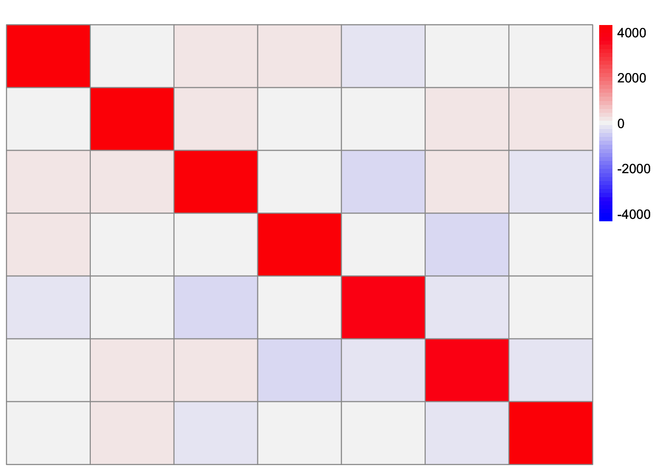
This is a heatmap of \(F'F\) where the diagonal entries are set to zero. (This is to get a sense of the scale of the off-diagonal entries):
FtF_minus_diag <- FtF
diag(FtF_minus_diag) <- 0
plot_heatmap(FtF_minus_diag, colors_range = c('blue','gray96','red'), brks = seq(-max(abs(FtF_minus_diag)), max(abs(FtF_minus_diag)), length.out = 50))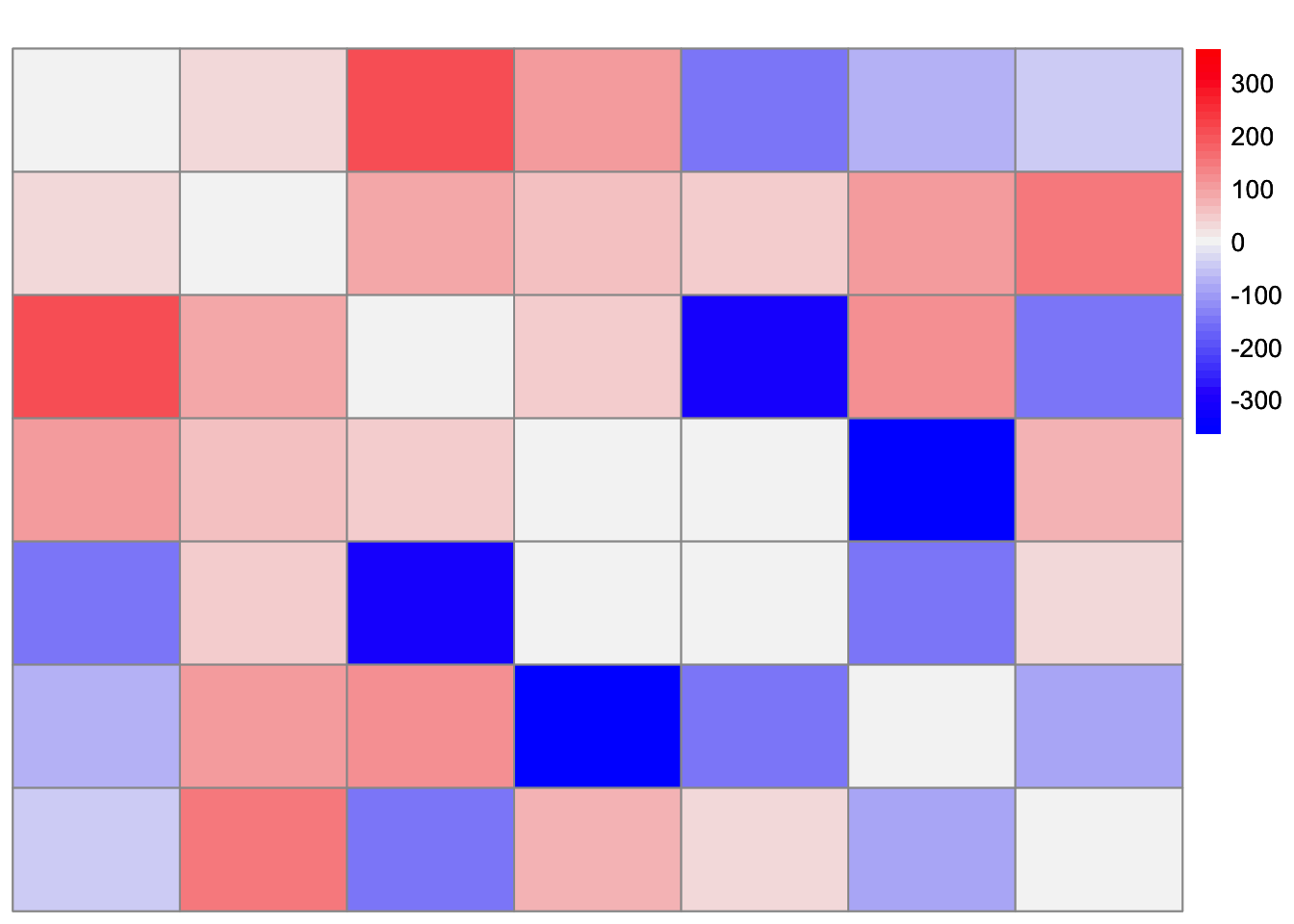
fitted_values <- (1/ncol(sim_data$Y))*sim_data$LL %*% diag(diag(FtF)) %*% t(sim_data$LL)
noise_mat <- sim_data$YYt - fitted_values

withf_fitted_values <- (1/ncol(sim_data$Y))*tcrossprod(tcrossprod(sim_data$LL, sim_data$FF))
withf_noise_mat <- sim_data$YYt - withf_fitted_values
This is a heatmap of the scaled Gram matrix, \(S = \frac{1}{p}XX'\):
plot_heatmap(sim_data$YYt, colors_range = c('blue','gray96','red'), brks = seq(-max(abs(sim_data$YYt)), max(abs(sim_data$YYt)), length.out = 50))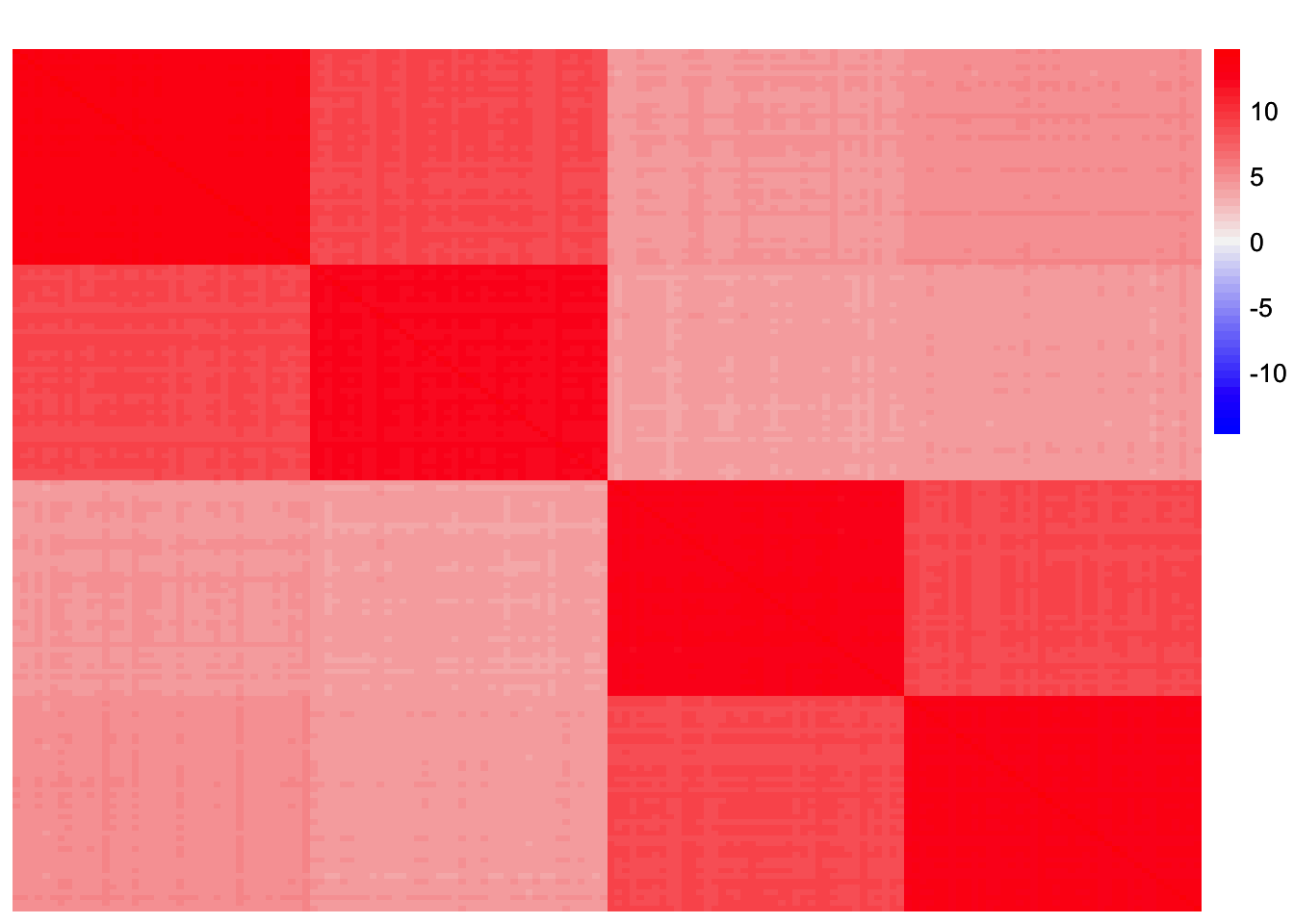
This is a heatmap of \(\frac{1}{p}LL'\) where \(L\) is appropriately scaled such that \(S \approx LL'\):
plot_heatmap(fitted_values, colors_range = c('blue','gray96','red'), brks = seq(-max(abs(fitted_values)), max(abs(fitted_values)), length.out = 50))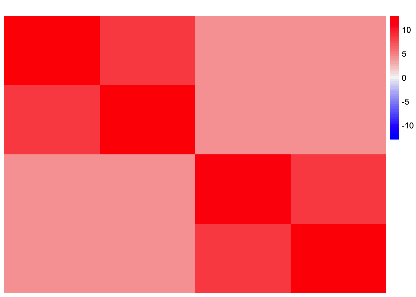
This is a heatmap of \(S - LL'\):
plot_heatmap(noise_mat, colors_range = c('blue','gray96','red'), brks = seq(-max(abs(noise_mat)), max(abs(noise_mat)), length.out = 50))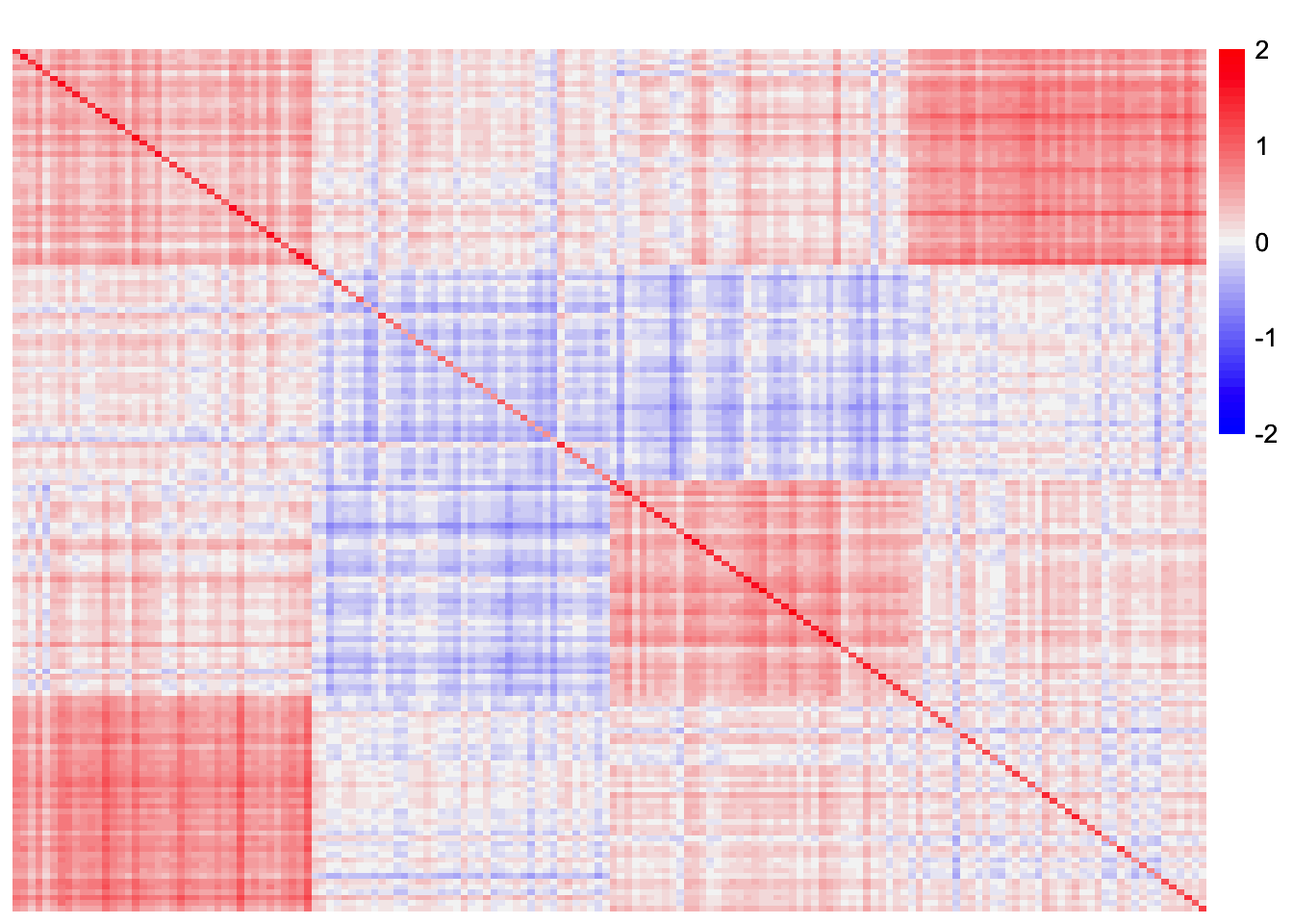
This is a heatmap of \(\frac{1}{p}LF'FL'\) (the scaling on \(L\) here may be different from the scaling on \(L\) in the previous construction):
plot_heatmap(withf_fitted_values, colors_range = c('blue','gray96','red'), brks = seq(-max(abs(withf_fitted_values)), max(abs(withf_fitted_values)), length.out = 50))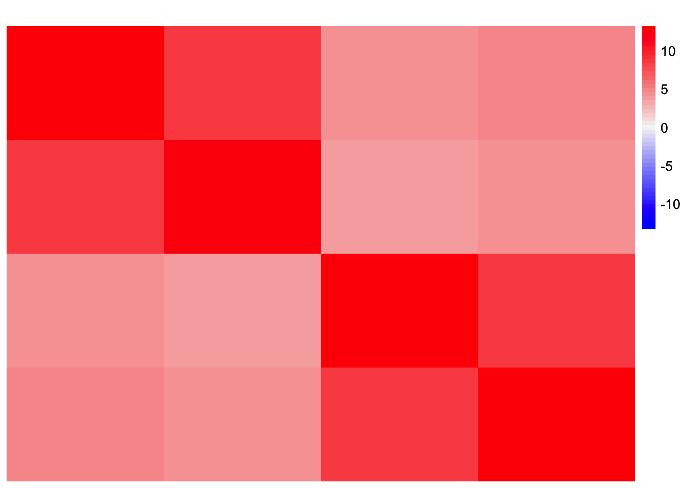
This is a heatmap of \(S - \frac{1}{p}LF'FL'\):
plot_heatmap(withf_noise_mat, colors_range = c('blue','gray96','red'), brks = seq(-max(abs(withf_noise_mat)), max(abs(withf_noise_mat)), length.out = 50))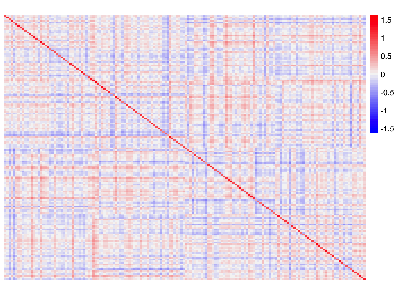
It seems like some of the off-diagonal entries in \(F'F\) contribute to a small level of correlation between groups 1 and 4 that is apparent in the scaled Gram matrix. So my guess is that symEBcovMF is trying to fit this structure, and thus chooses to group together the effects of group 1 and group 4.
What if I generate data with orthogonal F?
Here, I generate the data with an orthogonal \(F\) matrix. I picked a particular example where symEBcovMF with generalized binary does not yield the desired loadings estimate.
sim_args_orthog = list(pop_sizes = rep(40, 4), n_genes = 1000, branch_sds = rep(2,7), indiv_sd = 1, seed = 6, constrain_F = TRUE)
sim_data_orthog <- sim_4pops(sim_args_orthog)
This is a heatmap of the scaled Gram matrix:
plot_heatmap(sim_data_orthog$YYt, colors_range = c('blue','gray96','red'), brks = seq(-max(abs(sim_data_orthog$YYt)), max(abs(sim_data_orthog$YYt)), length.out = 50))
This is a scatter plot of the true loadings matrix:
pop_vec <- c(rep('A', 40), rep('B', 40), rep('C', 40), rep('D', 40))
plot_loadings(sim_data_orthog$LL, pop_vec)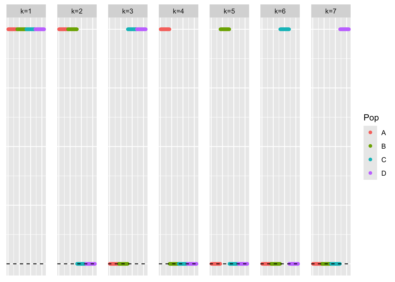
This is a plot of the eigenvalues of the Gram matrix:
S_orthog_eigen <- eigen(sim_data_orthog$YYt)
plot(S_orthog_eigen$values) + abline(a = 0, b = 0, col = 'red')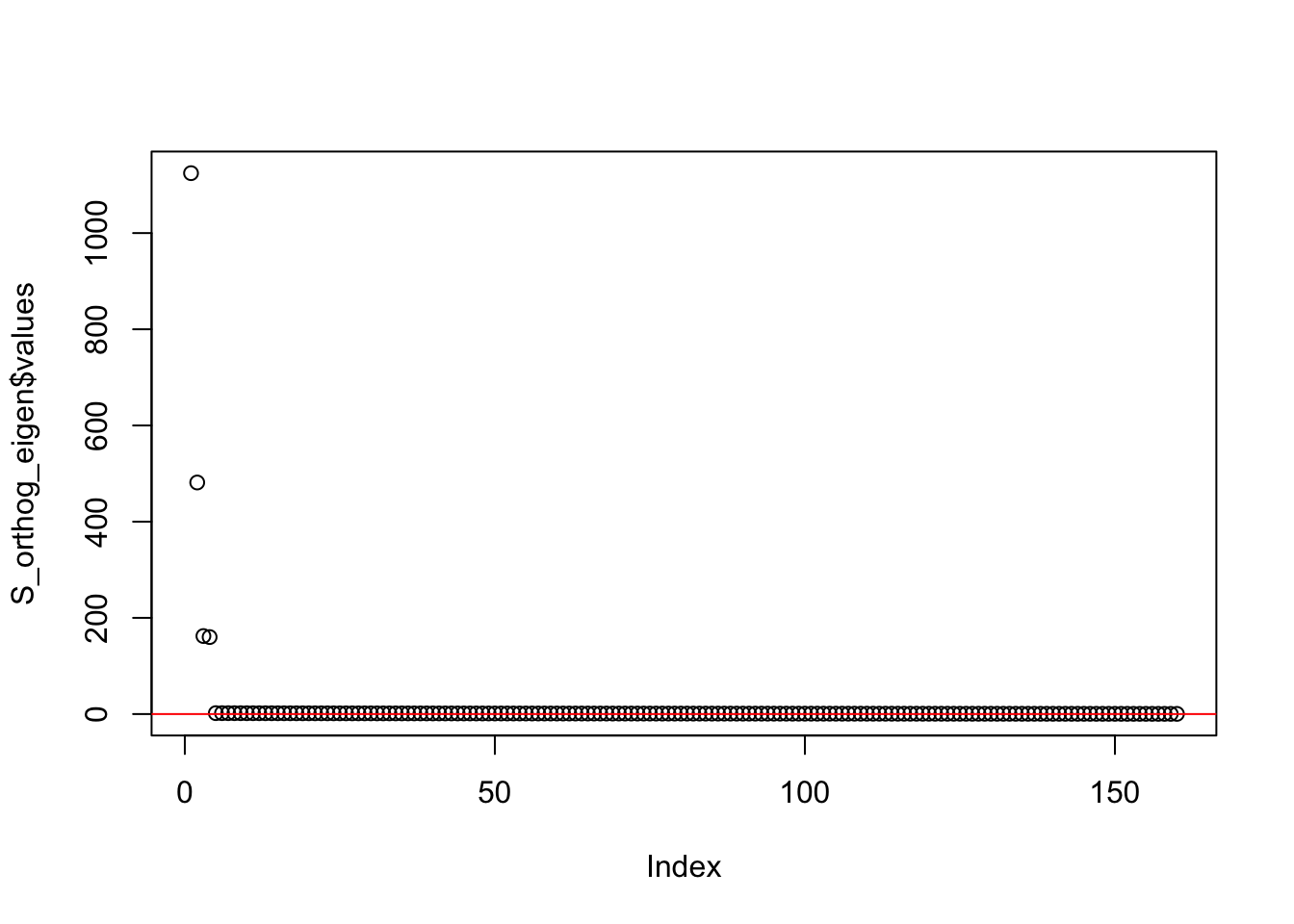
integer(0)This is the minimum eigenvalue:
min(S_orthog_eigen$values)[1] 0.3696272symEBcovMF with generalized binary prior
Here, we run symEBcovMF with generalized binary prior and
Kmax = 7:
symebcovmf_orthog_gb_rank7_fit <- sym_ebcovmf_fit(S = sim_data_orthog$YYt, ebnm_fn = ebnm::ebnm_generalized_binary, K = 7, maxiter = 500, rank_one_tol = 10^(-8), tol = 10^(-8), refit_lam = TRUE)[1] "elbo decreased by 0.0115381182476995"
[1] "elbo decreased by 0.054343875417544"
[1] "elbo decreased by 0.000618491005297983"
[1] "elbo decreased by 3.92901711165905e-10"This is a plot of the loadings estimate:
plot_loadings(symebcovmf_orthog_gb_rank7_fit$L_pm %*% diag(sqrt(symebcovmf_orthog_gb_rank7_fit$lambda)), pop_vec)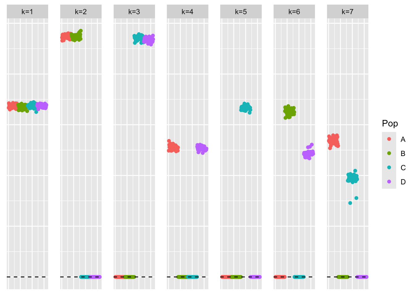
The loadings estimate does not follow a tree structure. In particular, the method does not find four single population effect factors. It finds factors which group together two population effects.
Residual Matrix example
Now, we run the procedure for the residual matrix example we’ve been
working with. First, we run symEBcovMF with generalized binary prior and
Kmax = 3 to fit the first three factors.
symebcovmf_orthog_gb_fit <- sym_ebcovmf_fit(S = sim_data_orthog$YYt, ebnm_fn = ebnm::ebnm_generalized_binary, K = 3, maxiter = 500, rank_one_tol = 10^(-8), tol = 10^(-8), refit_lam = TRUE)[1] "elbo decreased by 0.0115381182476995"
[1] "elbo decreased by 0.054343875417544"This is a plot of the estimates for the first three factors.
plot_loadings(symebcovmf_orthog_gb_fit$L_pm %*% diag(sqrt(symebcovmf_orthog_gb_fit$lambda)), pop_vec)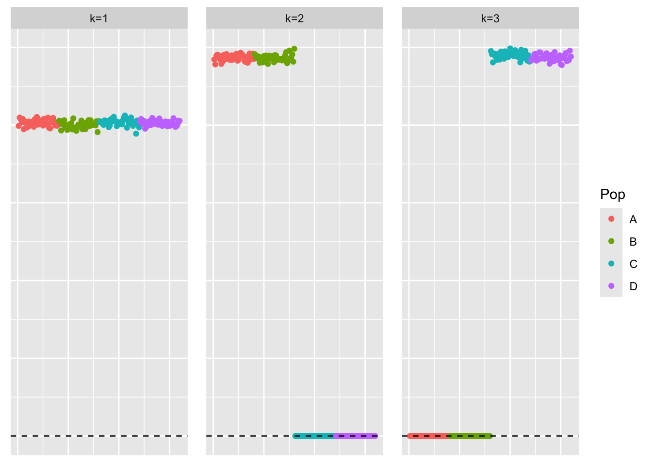
Now, we compute the residual matrix \(R = S - \sum_{k=1}^{3} \hat{\lambda}_k \hat{\ell}_3 \hat{\ell}_3'\):
rank3_orthog_resid_matrix <- sim_data_orthog$YYt - tcrossprod(symebcovmf_orthog_gb_fit$L_pm %*% diag(sqrt(symebcovmf_orthog_gb_fit$lambda)))This is a heatmap of the residual matrix, \(R\):
plot_heatmap(rank3_orthog_resid_matrix, colors_range = c('blue','gray96','red'), brks = seq(-max(abs(rank3_orthog_resid_matrix)), max(abs(rank3_orthog_resid_matrix)), length.out = 50))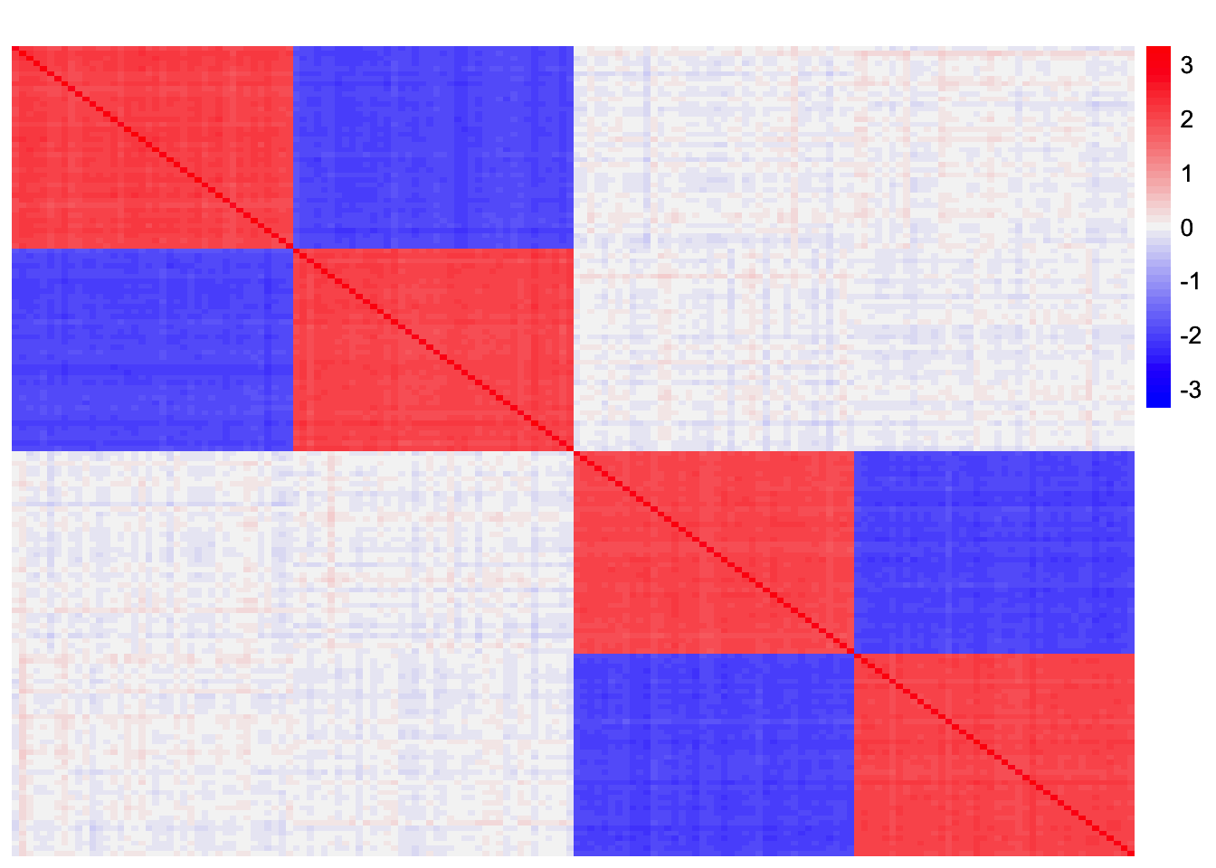
Now, we fit a fourth factor using a point-exponential prior.
symebcovmf_orthog_gb_exp_fac4_fit <- sym_ebcovmf_r1_fit(sim_data_orthog$YYt, symebcovmf_orthog_gb_fit, ebnm_fn = ebnm_point_exponential, maxiter = 100, tol = 10^(-8))This is a plot of the estimate for the fourth factor.
plot(symebcovmf_orthog_gb_exp_fac4_fit$L_pm[,4], ylab = 'Fourth Factor')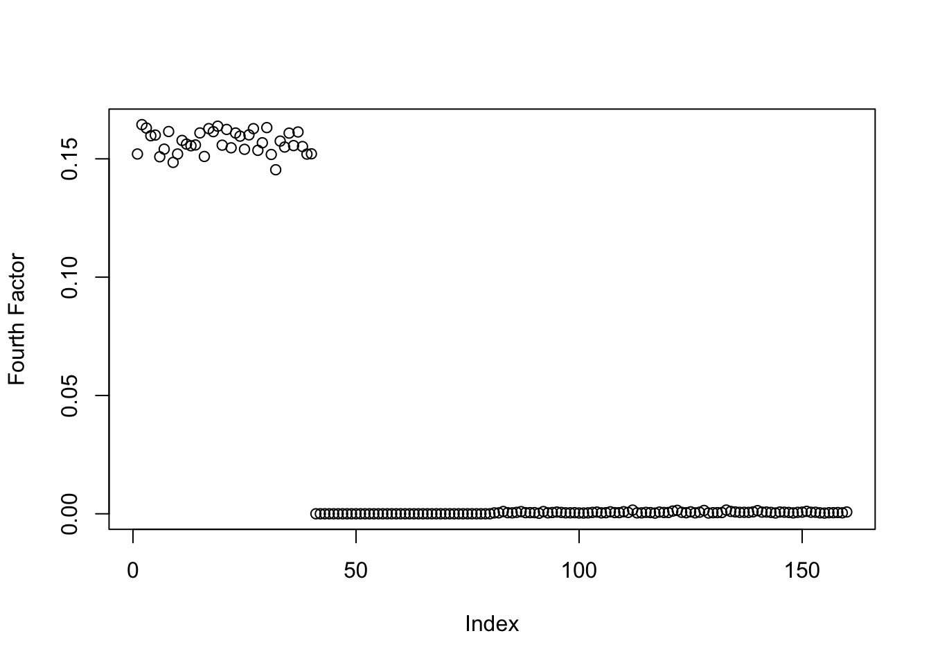
In this example, the point-exponential prior for the fourth factor does find the single effect factor. This seems to suggest that even mild correlations in the \(F\) matrix can sway the method, causing it to recover structure that is not really interesting to us. My guess is that other methods like GBCD can overcome this issue through backfitting.
sessionInfo()R version 4.3.2 (2023-10-31)
Platform: aarch64-apple-darwin20 (64-bit)
Running under: macOS Sonoma 14.4.1
Matrix products: default
BLAS: /Library/Frameworks/R.framework/Versions/4.3-arm64/Resources/lib/libRblas.0.dylib
LAPACK: /Library/Frameworks/R.framework/Versions/4.3-arm64/Resources/lib/libRlapack.dylib; LAPACK version 3.11.0
locale:
[1] en_US.UTF-8/en_US.UTF-8/en_US.UTF-8/C/en_US.UTF-8/en_US.UTF-8
time zone: America/Chicago
tzcode source: internal
attached base packages:
[1] stats graphics grDevices utils datasets methods base
other attached packages:
[1] ggplot2_3.5.1 pheatmap_1.0.12 ebnm_1.1-34 workflowr_1.7.1
loaded via a namespace (and not attached):
[1] gtable_0.3.5 xfun_0.48 bslib_0.8.0 processx_3.8.4
[5] lattice_0.22-6 callr_3.7.6 vctrs_0.6.5 tools_4.3.2
[9] ps_1.7.7 generics_0.1.3 tibble_3.2.1 fansi_1.0.6
[13] highr_0.11 pkgconfig_2.0.3 Matrix_1.6-5 SQUAREM_2021.1
[17] RColorBrewer_1.1-3 lifecycle_1.0.4 truncnorm_1.0-9 farver_2.1.2
[21] compiler_4.3.2 stringr_1.5.1 git2r_0.33.0 munsell_0.5.1
[25] getPass_0.2-4 httpuv_1.6.15 htmltools_0.5.8.1 sass_0.4.9
[29] yaml_2.3.10 later_1.3.2 pillar_1.9.0 jquerylib_0.1.4
[33] whisker_0.4.1 cachem_1.1.0 trust_0.1-8 RSpectra_0.16-2
[37] tidyselect_1.2.1 digest_0.6.37 stringi_1.8.4 dplyr_1.1.4
[41] ashr_2.2-66 labeling_0.4.3 splines_4.3.2 rprojroot_2.0.4
[45] fastmap_1.2.0 grid_4.3.2 colorspace_2.1-1 cli_3.6.3
[49] invgamma_1.1 magrittr_2.0.3 utf8_1.2.4 withr_3.0.1
[53] scales_1.3.0 promises_1.3.0 horseshoe_0.2.0 rmarkdown_2.28
[57] httr_1.4.7 deconvolveR_1.2-1 evaluate_1.0.0 knitr_1.48
[61] irlba_2.3.5.1 rlang_1.1.4 Rcpp_1.0.13 mixsqp_0.3-54
[65] glue_1.8.0 rstudioapi_0.16.0 jsonlite_1.8.9 R6_2.5.1
[69] fs_1.6.4