symebcovmf_binary_tree_resid_exploration
Annie Xie
2025-04-30
Last updated: 2025-05-02
Checks: 7 0
Knit directory:
symmetric_covariance_decomposition/
This reproducible R Markdown analysis was created with workflowr (version 1.7.1). The Checks tab describes the reproducibility checks that were applied when the results were created. The Past versions tab lists the development history.
Great! Since the R Markdown file has been committed to the Git repository, you know the exact version of the code that produced these results.
Great job! The global environment was empty. Objects defined in the global environment can affect the analysis in your R Markdown file in unknown ways. For reproduciblity it’s best to always run the code in an empty environment.
The command set.seed(20250408) was run prior to running
the code in the R Markdown file. Setting a seed ensures that any results
that rely on randomness, e.g. subsampling or permutations, are
reproducible.
Great job! Recording the operating system, R version, and package versions is critical for reproducibility.
Nice! There were no cached chunks for this analysis, so you can be confident that you successfully produced the results during this run.
Great job! Using relative paths to the files within your workflowr project makes it easier to run your code on other machines.
Great! You are using Git for version control. Tracking code development and connecting the code version to the results is critical for reproducibility.
The results in this page were generated with repository version 846345d. See the Past versions tab to see a history of the changes made to the R Markdown and HTML files.
Note that you need to be careful to ensure that all relevant files for
the analysis have been committed to Git prior to generating the results
(you can use wflow_publish or
wflow_git_commit). workflowr only checks the R Markdown
file, but you know if there are other scripts or data files that it
depends on. Below is the status of the Git repository when the results
were generated:
Ignored files:
    Ignored:    .DS_Store
    Ignored:    .Rhistory

Untracked files:
    Untracked:  analysis/symebcovmf_binary_tree_resid_orthog_exploration.Rmd
    Untracked:  analysis/unbal_nonoverlap_exploration.Rmd

Unstaged changes:
    Modified:   analysis/unbal_nonoverlap.Rmd
Note that any generated files, e.g. HTML, png, CSS, etc., are not included in this status report because it is ok for generated content to have uncommitted changes.
These are the previous versions of the repository in which changes were
made to the R Markdown
(analysis/symebcovmf_binary_tree_resid_exploration.Rmd) and
HTML (docs/symebcovmf_binary_tree_resid_exploration.html)
files. If you’ve configured a remote Git repository (see
?wflow_git_remote), click on the hyperlinks in the table
below to view the files as they were in that past version.
| File | Version | Author | Date | Message |
|---|---|---|---|---|
| Rmd | 846345d | Annie Xie | 2025-05-02 | Add text to residual matrix example |
| html | a1149d8 | Annie Xie | 2025-05-02 | Build site. |
| Rmd | 818d4cf | Annie Xie | 2025-05-02 | Edit text in residual matrix example analysis |
| html | 9ddb9f2 | Annie Xie | 2025-05-01 | Build site. |
| Rmd | 03b6512 | Annie Xie | 2025-05-01 | Edit observations in residual matrix example |
| html | 9a7a4f4 | Annie Xie | 2025-05-01 | Build site. |
| Rmd | f3ba89f | Annie Xie | 2025-05-01 | Add exploration of binary priors in tree residual matrix example |
Introduction
In this analysis, I am interested in exploring symEBcovMF with the generalized binary prior in the tree setting. This analysis will focus on the residual matrix example that I investigated in a different analysis.
Motivation
When applying symEBcovMF with generalized binary prior to tree data, I found that instead of population effect factors, the method would group two population effects together. I tried using the point-exponential prior to remedy this, but found that the point-exponential prior also found factors which grouped two population effects. After further exploring this, I found that the method preferred the factor with two population effects – when initialized from the true population effect factor, the method still converged to the factor with two population effects. In this analysis, I am interested in exploring the following question: if the prior is more strictly binary, will the rank-one fit with point-exponential prior find a single population effect factor for the fourth factor?
Packages and Functions
library(ebnm)
library(pheatmap)
library(ggplot2)
source('code/visualization_functions.R')
source('code/symebcovmf_functions.R')Data Generation
sim_4pops <- function(args) {
  set.seed(args$seed)

  n <- sum(args$pop_sizes)
  p <- args$n_genes

  FF <- matrix(rnorm(7 * p, sd = rep(args$branch_sds, each = p)), ncol = 7)
  # if (args$constrain_F) {
  #   FF_svd <- svd(FF)
  #   FF <- FF_svd$u
  #   FF <- t(t(FF) * branch_sds * sqrt(p))
  # }

  LL <- matrix(0, nrow = n, ncol = 7)
  LL[, 1] <- 1
  LL[, 2] <- rep(c(1, 1, 0, 0), times = args$pop_sizes)
  LL[, 3] <- rep(c(0, 0, 1, 1), times = args$pop_sizes)
  LL[, 4] <- rep(c(1, 0, 0, 0), times = args$pop_sizes)
  LL[, 5] <- rep(c(0, 1, 0, 0), times = args$pop_sizes)
  LL[, 6] <- rep(c(0, 0, 1, 0), times = args$pop_sizes)
  LL[, 7] <- rep(c(0, 0, 0, 1), times = args$pop_sizes)

  E <- matrix(rnorm(n * p, sd = args$indiv_sd), nrow = n)
  Y <- LL %*% t(FF) + E
  YYt <- (1/p)*tcrossprod(Y)
  return(list(Y = Y, YYt = YYt, LL = LL, FF = FF, K = ncol(LL)))
}
sim_args = list(pop_sizes = rep(40, 4), n_genes = 1000, branch_sds = rep(2,7), indiv_sd = 1, seed = 1)
sim_data <- sim_4pops(sim_args)This is a heatmap of the scaled Gram matrix:
plot_heatmap(sim_data$YYt, colors_range = c('blue','gray96','red'), brks = seq(-max(abs(sim_data$YYt)), max(abs(sim_data$YYt)), length.out = 50))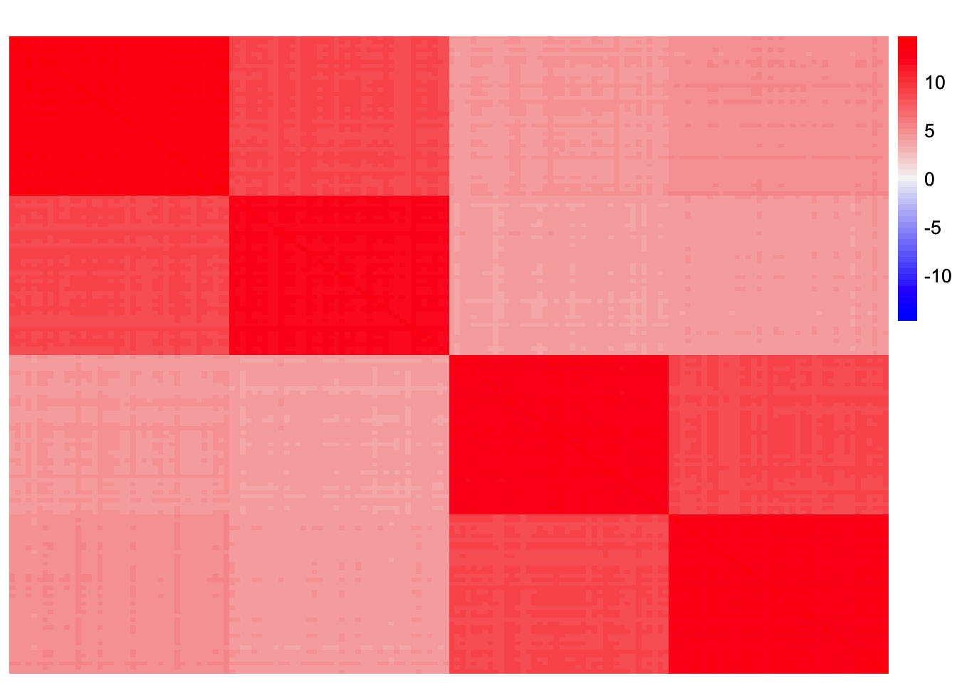
| Version | Author | Date |
|---|---|---|
| 9a7a4f4 | Annie Xie | 2025-05-01 |
This is a scatter plot of the true loadings matrix:
pop_vec <- c(rep('A', 40), rep('B', 40), rep('C', 40), rep('D', 40))
plot_loadings(sim_data$LL, pop_vec)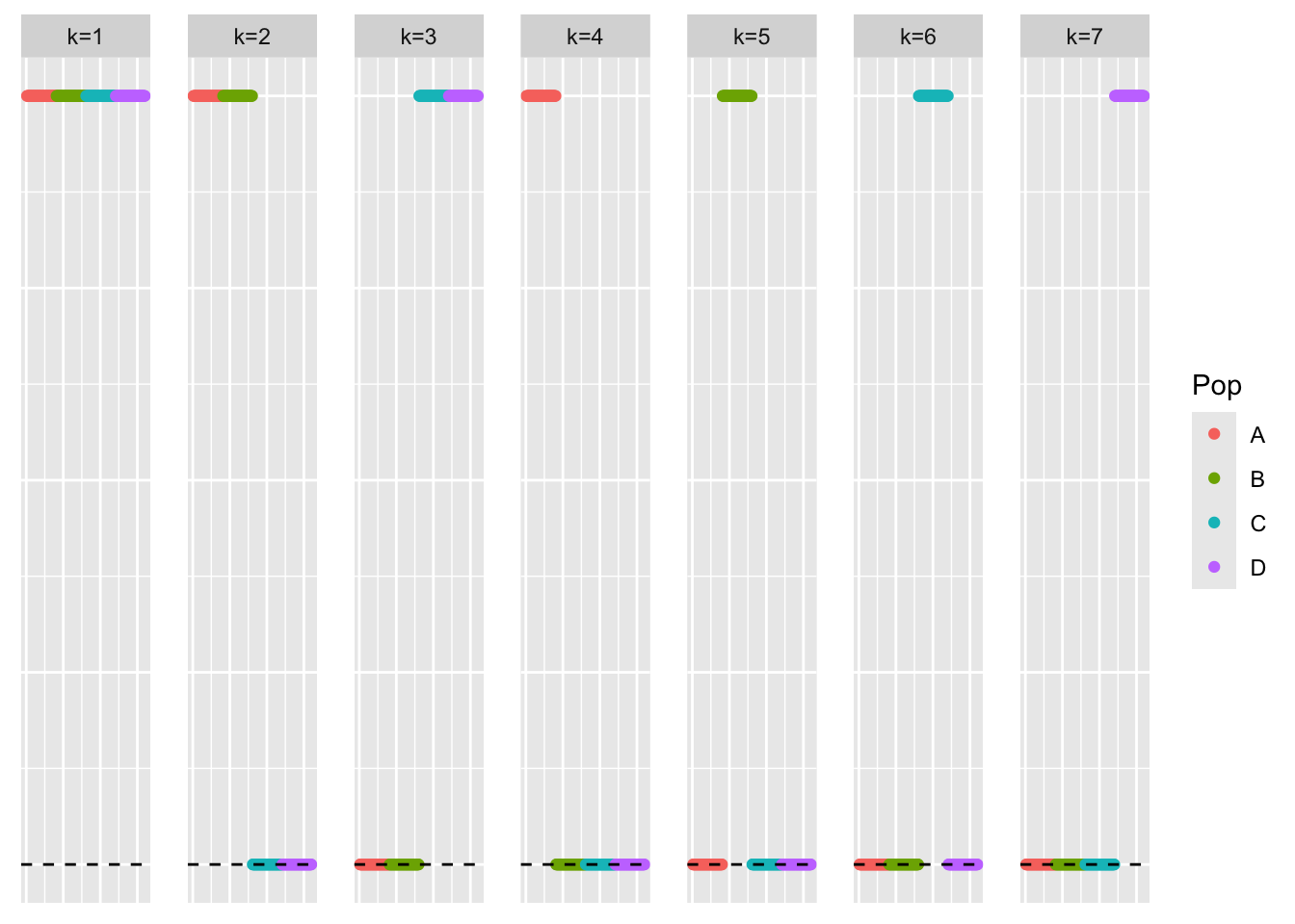
| Version | Author | Date |
|---|---|---|
| 9a7a4f4 | Annie Xie | 2025-05-01 |
This is a plot of the eigenvalues of the Gram matrix:
S_eigen <- eigen(sim_data$YYt)
plot(S_eigen$values) + abline(a = 0, b = 0, col = 'red')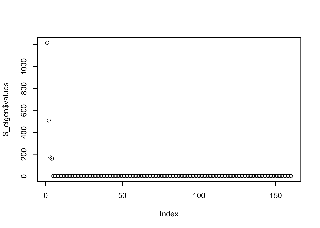
| Version | Author | Date |
|---|---|---|
| 9a7a4f4 | Annie Xie | 2025-05-01 |
integer(0)This is the minimum eigenvalue:
min(S_eigen$values)[1] 0.3724341Generalized binary with different scale parameter
First, I will try generalized binary prior with a different
scale parameter. The scale parameter refers to
the ratio \(\sigma/mu\). If the ratio
is small, then the prior will be closer to a strictly binary prior.
ebnm_generalized_binary_fix_scale <- function(x, s, mode = 'estimate', g_init = NULL, fix_g = FALSE, output = ebnm_output_default(), control = NULL){
  ebnm_gb_output <- ebnm::ebnm_generalized_binary(x = x, s = s, mode = mode,
                                                  scale = 0.01,
                                                  g_init = g_init, fix_g = fix_g,
                                                  output = output, control = control)
  return(ebnm_gb_output)
}
Residual Matrix
We construct the residual matrix from a fit of three factors.
symebcovmf_gb_fix_scale_rank3_fit <- sym_ebcovmf_fit(S = sim_data$YYt, ebnm_fn = ebnm_generalized_binary_fix_scale, K = 3, maxiter = 500, rank_one_tol = 10^(-8), tol = 10^(-8), refit_lam = TRUE)rank3_gb_fix_scale_resid_matrix <- sim_data$YYt - tcrossprod(symebcovmf_gb_fix_scale_rank3_fit$L_pm %*% diag(sqrt(symebcovmf_gb_fix_scale_rank3_fit$lambda)))This is a plot of the loadings estimate.
plot_loadings(symebcovmf_gb_fix_scale_rank3_fit$L_pm %*% diag(sqrt(symebcovmf_gb_fix_scale_rank3_fit$lambda)), pop_vec)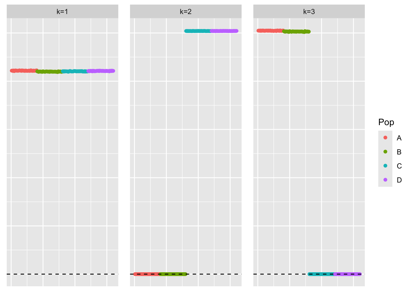
| Version | Author | Date |
|---|---|---|
| 9a7a4f4 | Annie Xie | 2025-05-01 |
This is a heatmap of the residual matrix.
plot_heatmap(rank3_gb_fix_scale_resid_matrix, colors_range = c('blue','gray96','red'), brks = seq(-max(abs(rank3_gb_fix_scale_resid_matrix)), max(abs(rank3_gb_fix_scale_resid_matrix)), length.out = 50))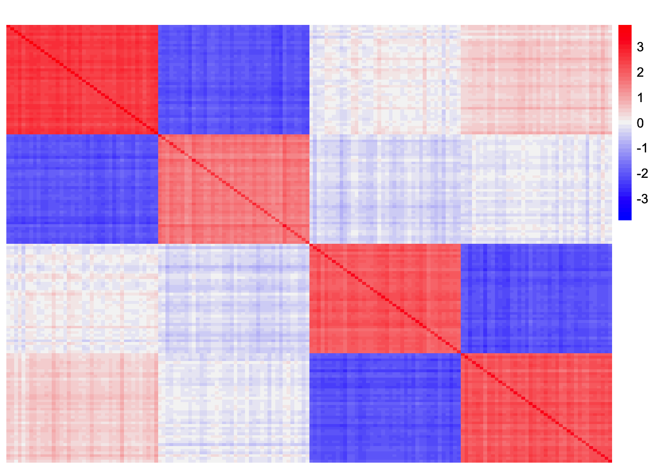
| Version | Author | Date |
|---|---|---|
| 9a7a4f4 | Annie Xie | 2025-05-01 |
Try fitting fourth factor with point-exponential prior
Now we try fitting a fourth factor using the rank-one fit with point-exponential prior.
symebcovmf_gb_fix_scale_exp_fac4_fit <- sym_ebcovmf_r1_fit(sim_data$YYt, symebcovmf_gb_fix_scale_rank3_fit, ebnm_fn = ebnm_point_exponential, maxiter = 100, tol = 10^(-8))This is a plot of the fourth factor estimate.
plot(symebcovmf_gb_fix_scale_exp_fac4_fit$L_pm[,4], ylab = 'Fourth Factor')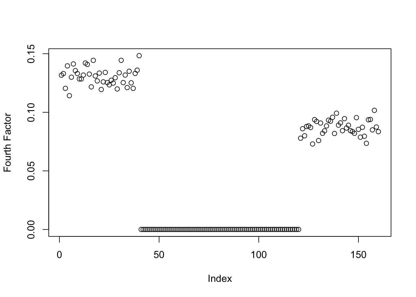
| Version | Author | Date |
|---|---|---|
| 9a7a4f4 | Annie Xie | 2025-05-01 |
This is a plot of the ELBO when optimizing the fourth factor.
fac4_idx <- which(symebcovmf_gb_fix_scale_exp_fac4_fit$vec_elbo_full == 4)
plot(symebcovmf_gb_fix_scale_exp_fac4_fit$vec_elbo_full[(fac4_idx+1): length(symebcovmf_gb_fix_scale_exp_fac4_fit$vec_elbo_full)], xlab = 'Iter', ylab = 'ELBO')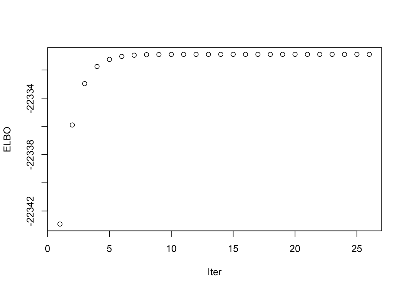
| Version | Author | Date |
|---|---|---|
| 9a7a4f4 | Annie Xie | 2025-05-01 |
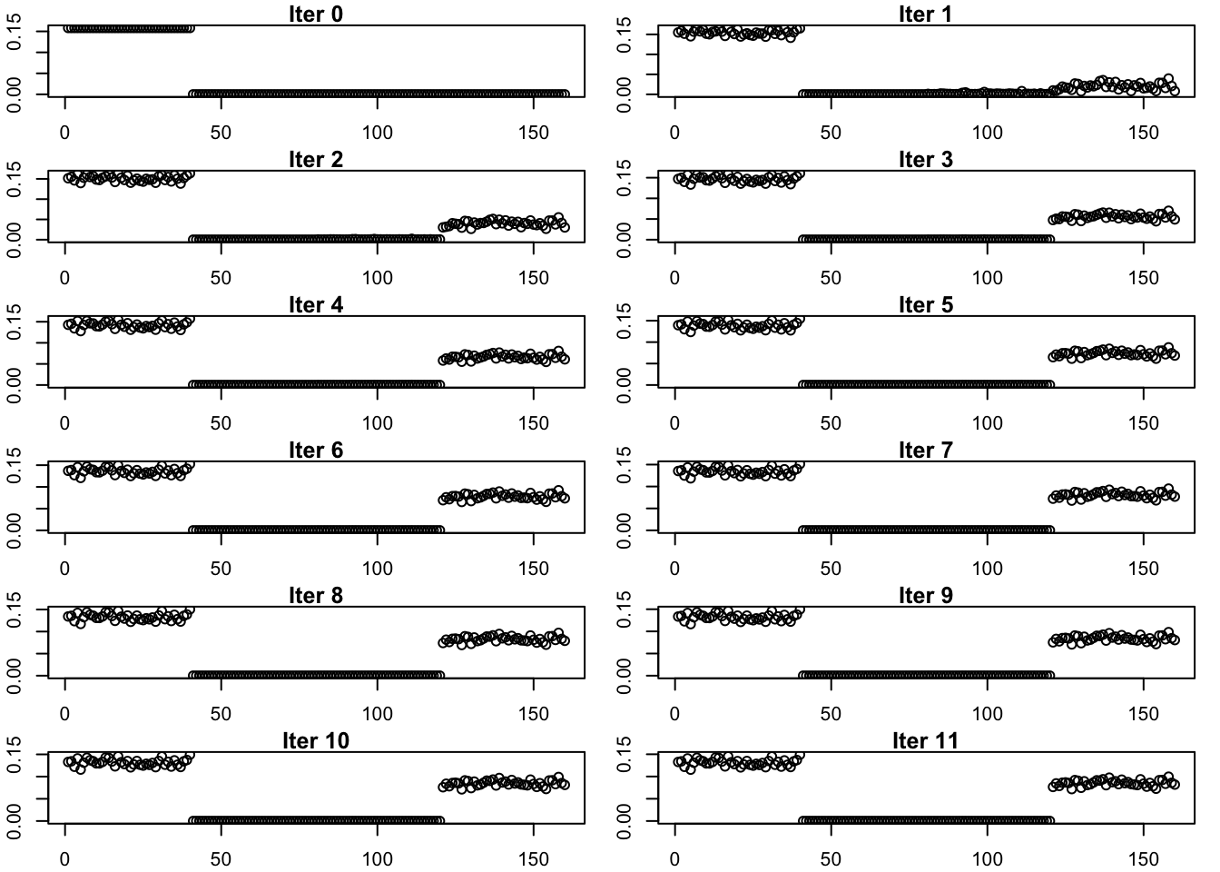
We see that the method still finds a factor with two population effects.
Progression of Estimate
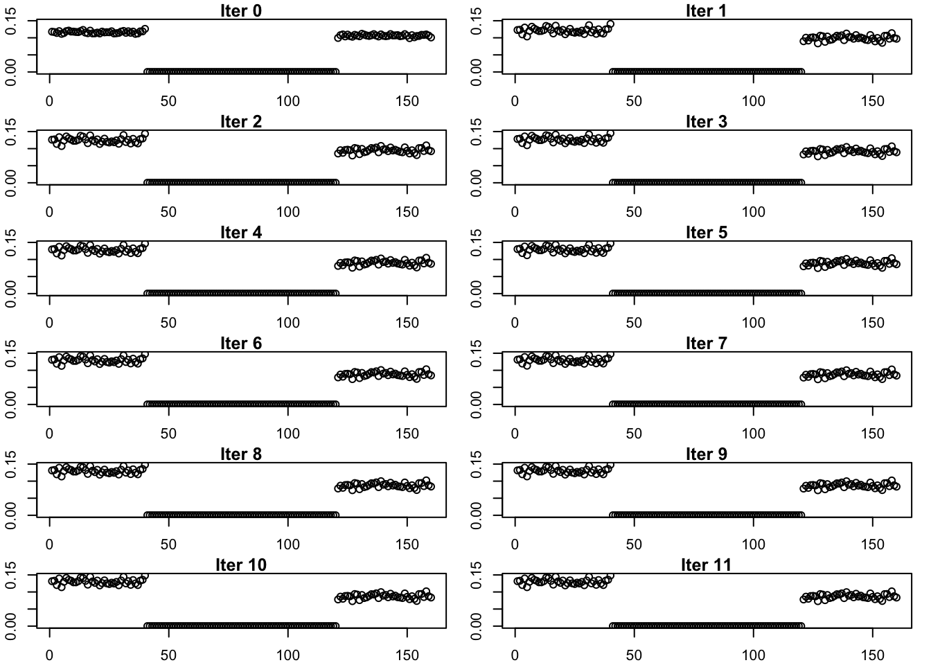
This is the progression of the estimate.
estimates_gb_fix_scale_exp_list <- list(sym_ebcovmf_r1_init(rank3_gb_fix_scale_resid_matrix)$v)
for (i in 1:11){
  estimates_gb_fix_scale_exp_list[[(i+1)]] <- sym_ebcovmf_r1_fit(sim_data$YYt, symebcovmf_gb_fix_scale_rank3_fit, ebnm_fn = ebnm_point_exponential, maxiter = i, tol = 10^(-8))$L_pm[,4]
}
par(mfrow = c(6,2), mar = c(2, 2, 1, 1) + 0.1)
max_y <- max(sapply(estimates_gb_fix_scale_exp_list, max))
min_y <- min(sapply(estimates_gb_fix_scale_exp_list, min))
for (i in 1:12){
plot(estimates_gb_fix_scale_exp_list[[i]], main = paste('Iter', (i-1)), ylab = 'L', ylim = c(min_y, max_y))
}
| Version | Author | Date |
|---|---|---|
| 9a7a4f4 | Annie Xie | 2025-05-01 |
par(mfrow = c(1,1))Try fitting fourth factor initialized at true factor
Now, I will try initializing with the true single population effect factor. This will help us determine if this is a convergence issue.
true_fac4 <- rep(c(1,0), times = c(40, 120))
true_fac4 <- true_fac4/sqrt(sum(true_fac4^2))
symebcovmf_gb_fix_scale_exp_true_init_fac4_fit <- sym_ebcovmf_r1_fit(sim_data$YYt, symebcovmf_gb_fix_scale_rank3_fit, ebnm_fn = ebnm_point_exponential, maxiter = 100, tol = 10^(-8), v_init = true_fac4)
This is a plot of the fourth factor estimate.
plot(symebcovmf_gb_fix_scale_exp_true_init_fac4_fit$L_pm[,4], ylab = 'Fourth Factor')
| Version | Author | Date |
|---|---|---|
| 9a7a4f4 | Annie Xie | 2025-05-01 |
This is a plot of the ELBO when optimizing the fourth factor.
fac4_idx <- which(symebcovmf_gb_fix_scale_exp_true_init_fac4_fit$vec_elbo_full == 4)
plot(symebcovmf_gb_fix_scale_exp_true_init_fac4_fit$vec_elbo_full[(fac4_idx+1): length(symebcovmf_gb_fix_scale_exp_true_init_fac4_fit$vec_elbo_full)], xlab = 'Iter', ylab = 'ELBO')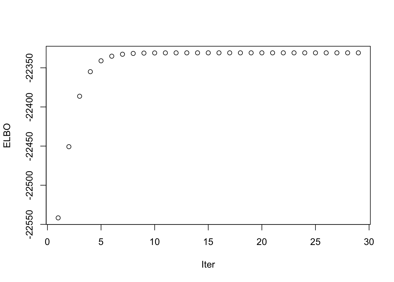
| Version | Author | Date |
|---|---|---|
| 9a7a4f4 | Annie Xie | 2025-05-01 |
We see that the method still converges to a factor with two population groups. This suggests this method prefers this factor as opposed to the single population effect factor.
Progression of Estimate
This is the progression of the estimate.
estimates_gb_fix_scale_exp_true_init_list <- list(true_fac4)
for (i in 1:11){
  estimates_gb_fix_scale_exp_true_init_list[[(i+1)]] <- sym_ebcovmf_r1_fit(sim_data$YYt, symebcovmf_gb_fix_scale_rank3_fit, ebnm_fn = ebnm_point_exponential, maxiter = i, tol = 10^(-8), v_init = rep(c(1,0), times = c(40, 120)))$L_pm[,4]
}
par(mfrow = c(6,2), mar = c(2, 2, 1, 1) + 0.1)
for (i in 1:12){
plot(estimates_gb_fix_scale_exp_true_init_list[[i]], main = paste('Iter', (i-1)), ylab = 'L')
}
| Version | Author | Date |
|---|---|---|
| 9a7a4f4 | Annie Xie | 2025-05-01 |
par(mfrow = c(1,1))Binormal Prior
Here, I will try the binormal prior. Given that changing the scale of the generalized binary prior didn’t work and it doesn’t appear to be a convergence issue, I don’t really expect this to perform much better. But it’s also possible this prior has better shrinkage or convergence properties, so maybe it will.
dbinormal = function (x,s,s0,lambda,log=TRUE){
  pi0 = 0.5
  pi1 = 0.5
  s2 = s^2
  s02 = s0^2
  l0 = dnorm(x,0,sqrt(lambda^2 * s02 + s2),log=TRUE)
  l1 = dnorm(x,lambda,sqrt(lambda^2 * s02 + s2),log=TRUE)
  logsum = log(pi0*exp(l0) + pi1*exp(l1))

  m = pmax(l0,l1)
  logsum = m + log(pi0*exp(l0-m) + pi1*exp(l1-m))
  if (log) return(sum(logsum))
  else return(exp(sum(logsum)))
}
ebnm_binormal = function(x,s, g_init = NULL, fix_g = FALSE, output = ebnm_output_default(), control = NULL){
# Add g_init to make the method run
if(is.null(dim(x)) == FALSE){
x <- c(x)
}
s0 = 0.01
lambda = optimize(function(lambda){-dbinormal(x,s,s0,lambda,log=TRUE)},
lower = 0, upper = max(x))$minimum
g = ashr::normalmix(pi=c(0.5,0.5), mean=c(0,lambda), sd=c(lambda * s0,lambda * s0))
postmean = ashr::postmean(g,ashr::set_data(x,s))
postsd = ashr::postsd(g,ashr::set_data(x,s))
log_likelihood <- ashr::calc_loglik(g, ashr::set_data(x,s))
return(list(fitted_g = g, posterior = data.frame(mean=postmean,sd=postsd), log_likelihood = log_likelihood))
}Residual Matrix
We construct the residual matrix from a fit of three factors.
symebcovmf_binormal_rank3_fit <- sym_ebcovmf_fit(S = sim_data$YYt, ebnm_fn = ebnm_binormal, K = 3, maxiter = 500, rank_one_tol = 10^(-8), tol = 10^(-8), refit_lam = TRUE)rank3_binormal_resid_matrix <- sim_data$YYt - tcrossprod(symebcovmf_binormal_rank3_fit$L_pm %*% diag(sqrt(symebcovmf_binormal_rank3_fit$lambda)))This is a plot of the loadings estimate.
plot_loadings(symebcovmf_binormal_rank3_fit$L_pm %*% diag(sqrt(symebcovmf_binormal_rank3_fit$lambda)), pop_vec)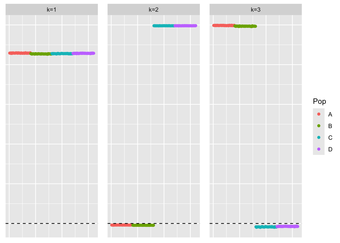
| Version | Author | Date |
|---|---|---|
| 9a7a4f4 | Annie Xie | 2025-05-01 |
This is a heatmap of the residual matrix.
plot_heatmap(rank3_binormal_resid_matrix, colors_range = c('blue','gray96','red'), brks = seq(-max(abs(rank3_binormal_resid_matrix)), max(abs(rank3_binormal_resid_matrix)), length.out = 50))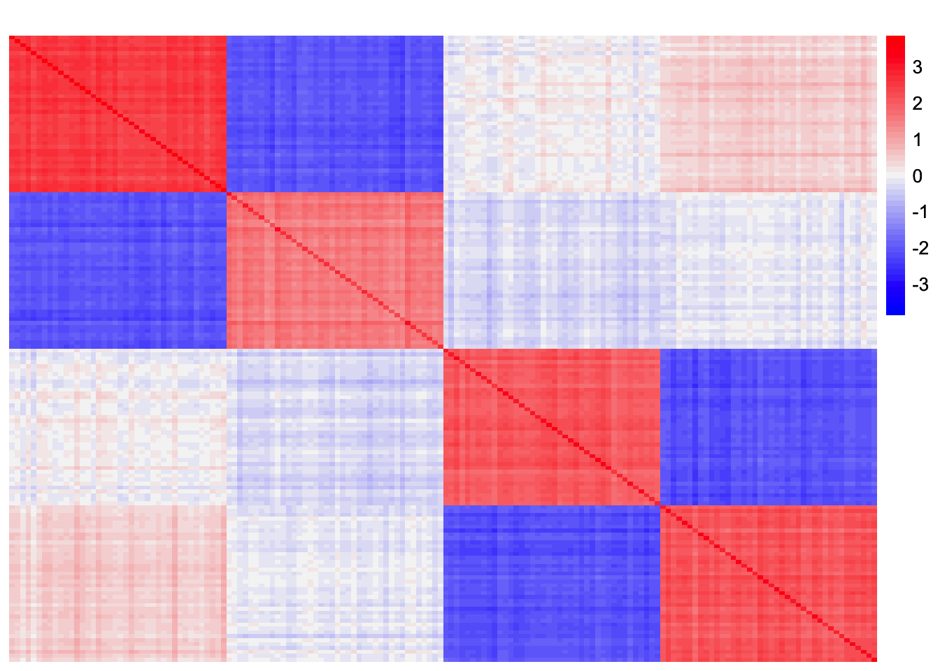
| Version | Author | Date |
|---|---|---|
| 9a7a4f4 | Annie Xie | 2025-05-01 |
Try fitting fourth factor with point-exponential prior
Now we try fitting a fourth factor using the rank-one fit with point-exponential prior.
symebcovmf_binormal_exp_fac4_fit <- sym_ebcovmf_r1_fit(sim_data$YYt, symebcovmf_binormal_rank3_fit, ebnm_fn = ebnm_point_exponential, maxiter = 100, tol = 10^(-8))This is a plot of the fourth factor estimate.
plot(symebcovmf_binormal_exp_fac4_fit$L_pm[,4], ylab = 'Fourth Factor')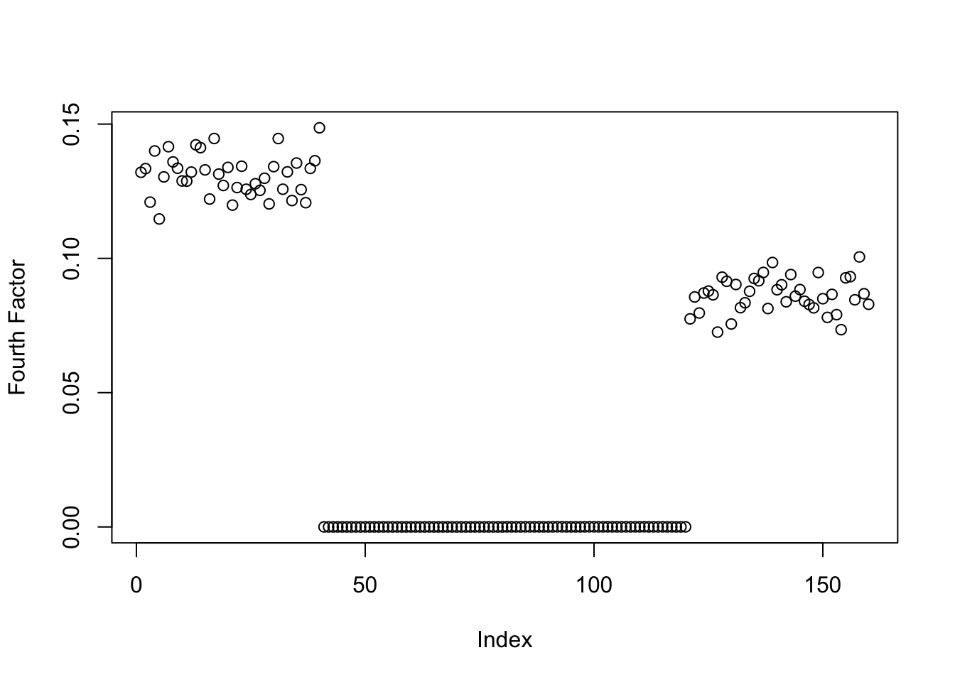
| Version | Author | Date |
|---|---|---|
| 9a7a4f4 | Annie Xie | 2025-05-01 |
This is a plot of the ELBO when optimizing the fourth factor.
fac4_idx <- which(symebcovmf_binormal_exp_fac4_fit$vec_elbo_full == 4)
plot(symebcovmf_binormal_exp_fac4_fit$vec_elbo_full[(fac4_idx+1): length(symebcovmf_binormal_exp_fac4_fit$vec_elbo_full)], xlab = 'Iter', ylab = 'ELBO')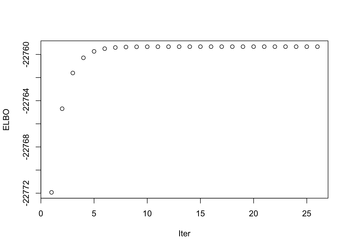
| Version | Author | Date |
|---|---|---|
| 9a7a4f4 | Annie Xie | 2025-05-01 |
Again, we see the method fits a factor with two population effects.
Progression of Estimate
This is the progression of the estimate.
estimates_binormal_exp_list <- list(sym_ebcovmf_r1_init(rank3_binormal_resid_matrix)$v)
for (i in 1:11){
  estimates_binormal_exp_list[[(i+1)]] <- sym_ebcovmf_r1_fit(sim_data$YYt, symebcovmf_binormal_rank3_fit, ebnm_fn = ebnm_point_exponential, maxiter = i, tol = 10^(-8))$L_pm[,4]
}
par(mfrow = c(6,2), mar = c(2, 2, 1, 1) + 0.1)
max_y <- max(sapply(estimates_binormal_exp_list, max))
min_y <- min(sapply(estimates_binormal_exp_list, min))
for (i in 1:12){
plot(estimates_binormal_exp_list[[i]], main = paste('Iter', (i-1)), ylab = 'L', ylim = c(min_y, max_y))
}
| Version | Author | Date |
|---|---|---|
| 9a7a4f4 | Annie Xie | 2025-05-01 |
par(mfrow = c(1,1))Try fitting fourth factor initialized at true factor
Now, I will try initializing with the true single population effect factor.
true_fac4 <- rep(c(1,0), times = c(40, 120))
true_fac4 <- true_fac4/sqrt(sum(true_fac4^2))
symebcovmf_binormal_exp_true_init_fac4_fit <- sym_ebcovmf_r1_fit(sim_data$YYt, symebcovmf_binormal_rank3_fit, ebnm_fn = ebnm_point_exponential, maxiter = 100, tol = 10^(-8), v_init = true_fac4)
This is a plot of the fourth factor estimate.
plot(symebcovmf_binormal_exp_true_init_fac4_fit$L_pm[,4], ylab = 'Fourth Factor')
| Version | Author | Date |
|---|---|---|
| 9a7a4f4 | Annie Xie | 2025-05-01 |
This is a plot of the ELBO when optimizing the fourth factor.
fac4_idx <- which(symebcovmf_binormal_exp_true_init_fac4_fit$vec_elbo_full == 4)
plot(symebcovmf_binormal_exp_true_init_fac4_fit$vec_elbo_full[(fac4_idx+1): length(symebcovmf_binormal_exp_true_init_fac4_fit$vec_elbo_full)], xlab = 'Iter', ylab = 'ELBO')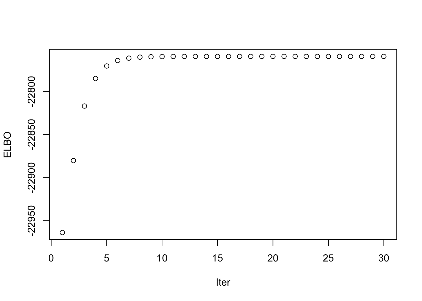
| Version | Author | Date |
|---|---|---|
| 9a7a4f4 | Annie Xie | 2025-05-01 |
Again, the method fits a factor with two population effects, suggesting it prefers this solution.
Progression of Estimate
This is the progression of the estimate.
estimates_binormal_exp_true_init_list <- list(true_fac4)
for (i in 1:11){
  estimates_binormal_exp_true_init_list[[(i+1)]] <- sym_ebcovmf_r1_fit(sim_data$YYt, symebcovmf_binormal_rank3_fit, ebnm_fn = ebnm_point_exponential, maxiter = i, tol = 10^(-8), v_init = rep(c(1,0), times = c(40, 120)))$L_pm[,4]
}
par(mfrow = c(6,2), mar = c(2, 2, 1, 1) + 0.1)
for (i in 1:12){
plot(estimates_binormal_exp_true_init_list[[i]], main = paste('Iter', (i-1)), ylab = 'L')
}
| Version | Author | Date |
|---|---|---|
| 9a7a4f4 | Annie Xie | 2025-05-01 |
par(mfrow = c(1,1))Observations
The results from all the priors are similar, and there is no evidence of convergence issues. This suggests that the strictness of the binary prior does not seem to help find single population effect factors for this dataset. Follow up hypotheses: Is the method picking up structure due to slight correlations in the columns of the \(F\) matrix? Or is the estimation of \(\lambda\) off, leaving behind structural components that should have been taken out?
sessionInfo()R version 4.3.2 (2023-10-31)
Platform: aarch64-apple-darwin20 (64-bit)
Running under: macOS Sonoma 14.4.1
Matrix products: default
BLAS: /Library/Frameworks/R.framework/Versions/4.3-arm64/Resources/lib/libRblas.0.dylib
LAPACK: /Library/Frameworks/R.framework/Versions/4.3-arm64/Resources/lib/libRlapack.dylib; LAPACK version 3.11.0
locale:
[1] en_US.UTF-8/en_US.UTF-8/en_US.UTF-8/C/en_US.UTF-8/en_US.UTF-8
time zone: America/Chicago
tzcode source: internal
attached base packages:
[1] stats graphics grDevices utils datasets methods base
other attached packages:
[1] ggplot2_3.5.1 pheatmap_1.0.12 ebnm_1.1-34 workflowr_1.7.1
loaded via a namespace (and not attached):
[1] gtable_0.3.5 xfun_0.48 bslib_0.8.0 processx_3.8.4
[5] lattice_0.22-6 callr_3.7.6 vctrs_0.6.5 tools_4.3.2
[9] ps_1.7.7 generics_0.1.3 tibble_3.2.1 fansi_1.0.6
[13] highr_0.11 pkgconfig_2.0.3 Matrix_1.6-5 SQUAREM_2021.1
[17] RColorBrewer_1.1-3 lifecycle_1.0.4 truncnorm_1.0-9 farver_2.1.2
[21] compiler_4.3.2 stringr_1.5.1 git2r_0.33.0 munsell_0.5.1
[25] getPass_0.2-4 httpuv_1.6.15 htmltools_0.5.8.1 sass_0.4.9
[29] yaml_2.3.10 later_1.3.2 pillar_1.9.0 jquerylib_0.1.4
[33] whisker_0.4.1 cachem_1.1.0 trust_0.1-8 RSpectra_0.16-2
[37] tidyselect_1.2.1 digest_0.6.37 stringi_1.8.4 dplyr_1.1.4
[41] ashr_2.2-66 labeling_0.4.3 splines_4.3.2 rprojroot_2.0.4
[45] fastmap_1.2.0 grid_4.3.2 colorspace_2.1-1 cli_3.6.3
[49] invgamma_1.1 magrittr_2.0.3 utf8_1.2.4 withr_3.0.1
[53] scales_1.3.0 promises_1.3.0 horseshoe_0.2.0 rmarkdown_2.28
[57] httr_1.4.7 deconvolveR_1.2-1 evaluate_1.0.0 knitr_1.48
[61] irlba_2.3.5.1 rlang_1.1.4 Rcpp_1.0.13 mixsqp_0.3-54
[65] glue_1.8.0 rstudioapi_0.16.0 jsonlite_1.8.9 R6_2.5.1
[69] fs_1.6.4