symebcovmf_binary_prior_tree_exploration
Annie Xie
2025-04-29
Last updated: 2025-05-01
Checks: 7 0
Knit directory:
symmetric_covariance_decomposition/
This reproducible R Markdown analysis was created with workflowr (version 1.7.1). The Checks tab describes the reproducibility checks that were applied when the results were created. The Past versions tab lists the development history.
Great! Since the R Markdown file has been committed to the Git repository, you know the exact version of the code that produced these results.
Great job! The global environment was empty. Objects defined in the global environment can affect the analysis in your R Markdown file in unknown ways. For reproduciblity it’s best to always run the code in an empty environment.
The command set.seed(20250408) was run prior to running
the code in the R Markdown file. Setting a seed ensures that any results
that rely on randomness, e.g. subsampling or permutations, are
reproducible.
Great job! Recording the operating system, R version, and package versions is critical for reproducibility.
Nice! There were no cached chunks for this analysis, so you can be confident that you successfully produced the results during this run.
Great job! Using relative paths to the files within your workflowr project makes it easier to run your code on other machines.
Great! You are using Git for version control. Tracking code development and connecting the code version to the results is critical for reproducibility.
The results in this page were generated with repository version 1a1bbf8. See the Past versions tab to see a history of the changes made to the R Markdown and HTML files.
Note that you need to be careful to ensure that all relevant files for
the analysis have been committed to Git prior to generating the results
(you can use wflow_publish or
wflow_git_commit). workflowr only checks the R Markdown
file, but you know if there are other scripts or data files that it
depends on. Below is the status of the Git repository when the results
were generated:
Ignored files:
    Ignored:    .DS_Store
    Ignored:    .Rhistory

Untracked files:
    Untracked:  analysis/symebcovmf_binary_tree_resid_exploration.Rmd
    Untracked:  analysis/symebcovmf_binary_tree_resid_orthog_exploration.Rmd
    Untracked:  analysis/unbal_nonoverlap_exploration.Rmd

Unstaged changes:
    Modified:   analysis/unbal_nonoverlap.Rmd
Note that any generated files, e.g. HTML, png, CSS, etc., are not included in this status report because it is ok for generated content to have uncommitted changes.
These are the previous versions of the repository in which changes were
made to the R Markdown
(analysis/symebcovmf_binary_prior_tree_exploration.Rmd) and
HTML (docs/symebcovmf_binary_prior_tree_exploration.html)
files. If you’ve configured a remote Git repository (see
?wflow_git_remote), click on the hyperlinks in the table
below to view the files as they were in that past version.
| File | Version | Author | Date | Message |
|---|---|---|---|---|
| Rmd | 1a1bbf8 | Annie Xie | 2025-05-01 | Add exploration of binary priors in tree setting |
Introduction
In this analysis, I am interested in exploring symEBcovMF with the generalized binary prior and other binary priors in the tree setting.
Motivation
When applying symEBcovMF with generalized binary prior to tree data, I found that instead of population effect factors, the method would group two population effects together. I tried using the point-exponential prior to remedy this, but found that the point-exponential prior also found factors which grouped two population effects. After further exploring this, I found that the method preferred the factor with two population effects – when initialized from the true population effect factor, the method still converged to the factor with two population effects. In this analysis, I am interested in other binary priors (binormal prior and generalized binary prior with different scales) and whether any of them yield a tree-structured loadings estimate.
Packages and Functions
library(ebnm)
library(pheatmap)
library(ggplot2)
source('code/visualization_functions.R')
source('code/symebcovmf_functions.R')Data Generation
sim_4pops <- function(args) {
  set.seed(args$seed)

  n <- sum(args$pop_sizes)
  p <- args$n_genes

  FF <- matrix(rnorm(7 * p, sd = rep(args$branch_sds, each = p)), ncol = 7)
  # if (args$constrain_F) {
  #   FF_svd <- svd(FF)
  #   FF <- FF_svd$u
  #   FF <- t(t(FF) * branch_sds * sqrt(p))
  # }

  LL <- matrix(0, nrow = n, ncol = 7)
  LL[, 1] <- 1
  LL[, 2] <- rep(c(1, 1, 0, 0), times = args$pop_sizes)
  LL[, 3] <- rep(c(0, 0, 1, 1), times = args$pop_sizes)
  LL[, 4] <- rep(c(1, 0, 0, 0), times = args$pop_sizes)
  LL[, 5] <- rep(c(0, 1, 0, 0), times = args$pop_sizes)
  LL[, 6] <- rep(c(0, 0, 1, 0), times = args$pop_sizes)
  LL[, 7] <- rep(c(0, 0, 0, 1), times = args$pop_sizes)

  E <- matrix(rnorm(n * p, sd = args$indiv_sd), nrow = n)
  Y <- LL %*% t(FF) + E
  YYt <- (1/p)*tcrossprod(Y)
  return(list(Y = Y, YYt = YYt, LL = LL, FF = FF, K = ncol(LL)))
}
sim_args = list(pop_sizes = rep(40, 4), n_genes = 1000, branch_sds = rep(2,7), indiv_sd = 1, seed = 1)
sim_data <- sim_4pops(sim_args)This is a heatmap of the scaled Gram matrix:
plot_heatmap(sim_data$YYt, colors_range = c('blue','gray96','red'), brks = seq(-max(abs(sim_data$YYt)), max(abs(sim_data$YYt)), length.out = 50))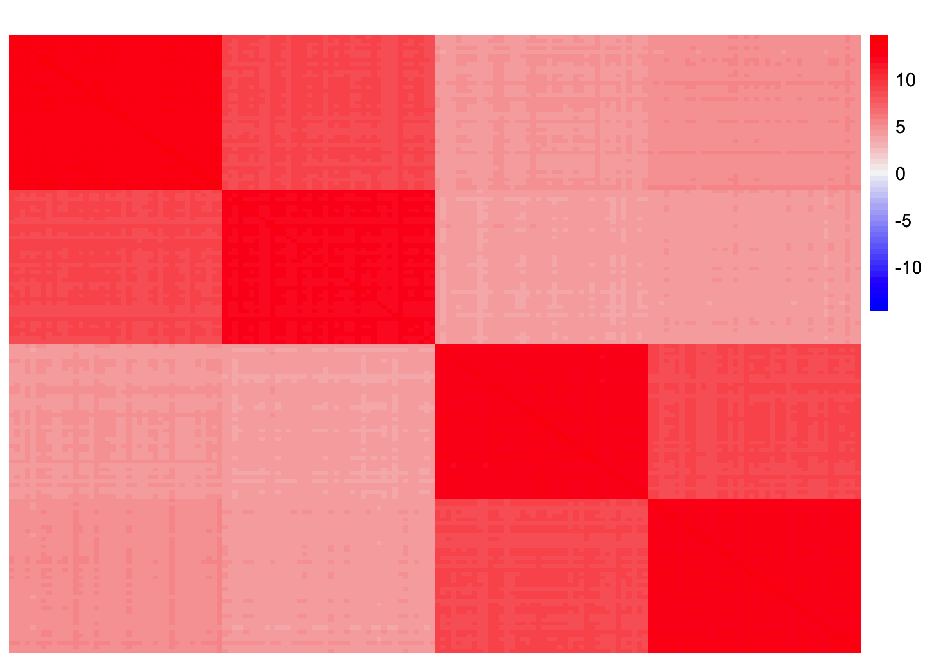
This is a scatter plot of the true loadings matrix:
pop_vec <- c(rep('A', 40), rep('B', 40), rep('C', 40), rep('D', 40))
plot_loadings(sim_data$LL, pop_vec)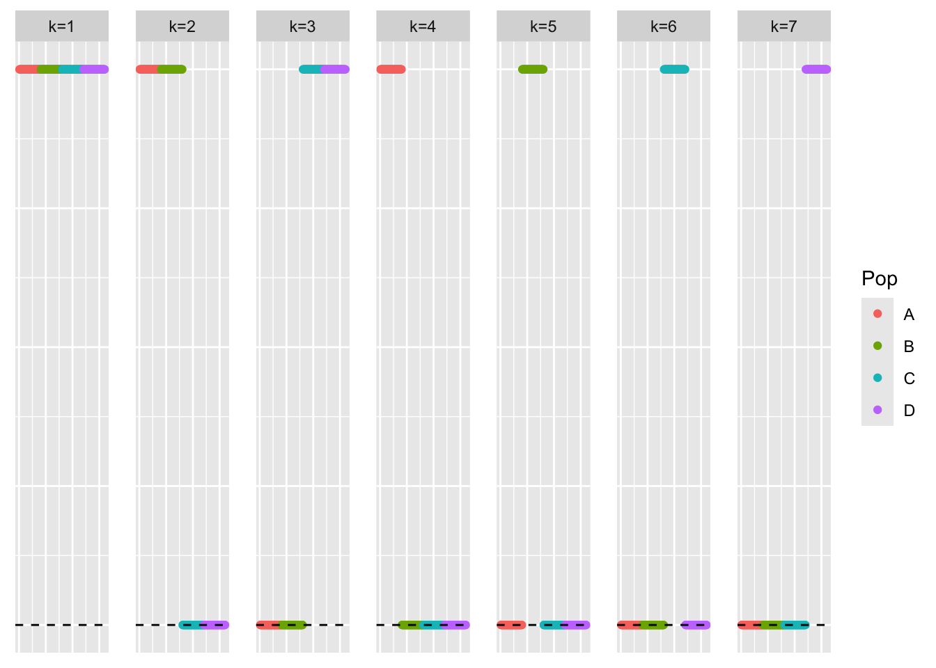
This is a plot of the eigenvalues of the Gram matrix:
S_eigen <- eigen(sim_data$YYt)
plot(S_eigen$values) + abline(a = 0, b = 0, col = 'red')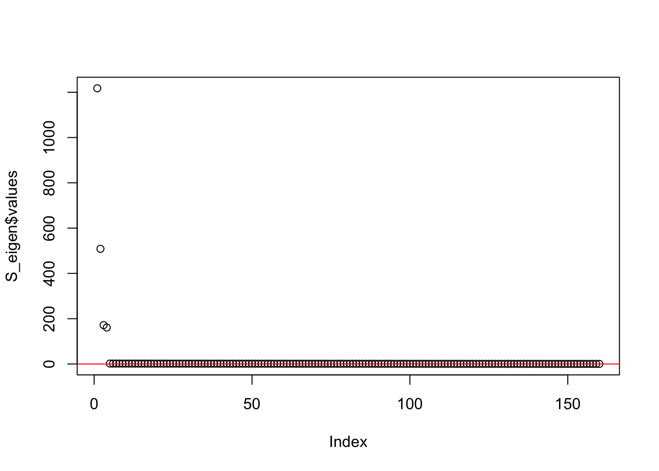
integer(0)This is the minimum eigenvalue:
min(S_eigen$values)[1] 0.3724341symEBcovMF with generalized binary prior
Here, we apply symEBcovMF with generalized binary prior (using the
default scale setting, scale - 0.1):
symebcovmf_gb_fit <- sym_ebcovmf_fit(S = sim_data$YYt, ebnm_fn = ebnm::ebnm_generalized_binary, K = 7, maxiter = 500, rank_one_tol = 10^(-8), tol = 10^(-8), refit_lam = TRUE)[1] "elbo decreased by 0.185693113584421"
[1] "elbo decreased by 0.0114876429142896"
[1] "elbo decreased by 1.5825207810849e-10"This is a plot of the loadings estimate:
plot_loadings(symebcovmf_gb_fit$L_pm %*% diag(sqrt(symebcovmf_gb_fit$lambda)), pop_vec)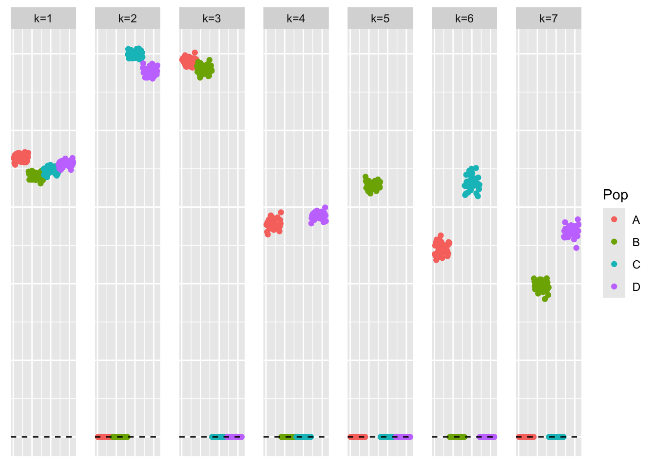
This is a plot of the estimate for the fourth factor:
plot(symebcovmf_gb_fit$L_pm[,4], ylab = 'Fourth Factor')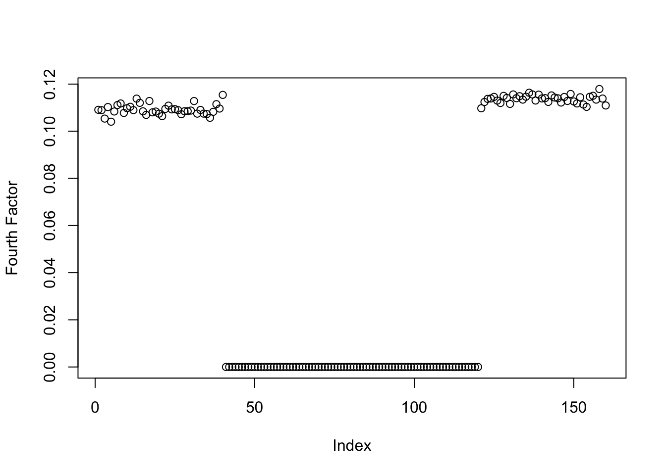
This is the ELBO:
symebcovmf_gb_fit$elbo[1] -14979.17As noted in our motivation, the estimate does not have four single population effect factors. It has one, but the other three factors group two population effects together. I have not looked into whether this is a convergence issue (i.e. does this solution have a higher ELBO than the desired solution?) or whether the method prefers this solution.
Alter ratio parameter of generalized binary
The first thing I will try is changing the scale
parameter in the generalized binary prior. The scale
parameter refers to the ratio \(\sigma/mu\). If the ratio is small, then
the prior will be closer to a strictly binary prior. The idea behind
this approach is to make the factors closer to binary in order to
prevent the “point of no return” where the method prefers to add factors
with grouped effects rather than sparse group effect factors.
ebnm_generalized_binary_fix_scale <- function(x, s, mode = 'estimate', g_init = NULL, fix_g = FALSE, output = ebnm_output_default(), control = NULL){
  ebnm_gb_output <- ebnm::ebnm_generalized_binary(x = x, s = s, mode = mode,
                                                  scale = 0.01,
                                                  g_init = g_init, fix_g = fix_g,
                                                  output = output, control = control)
  return(ebnm_gb_output)
}
symebcovmf_gb_fix_scale_fit <- sym_ebcovmf_fit(S = sim_data$YYt, ebnm_fn = ebnm_generalized_binary_fix_scale, K = 7, maxiter = 500, rank_one_tol = 10^(-8), tol = 10^(-8), refit_lam = TRUE)[1] "elbo decreased by 29.6132054929167"Note: There’s a very significant ELBO decrease when I run symEBcovMF with this prior. Previously, I had attributed ELBO decreases with the generalized binary prior to optimization issues. This is a note to myself to double check that. (Maybe we see ELBO decreases because the residual matrices are not positive definite?)
This is a plot of the loadings estimate:
plot_loadings(symebcovmf_gb_fix_scale_fit$L_pm %*% diag(sqrt(symebcovmf_gb_fix_scale_fit$lambda)), pop_vec)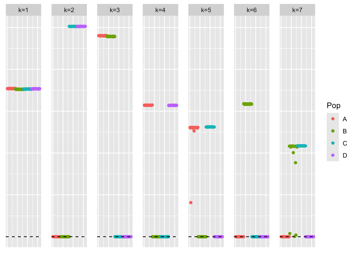
This is a plot of the estimate for the fourth factor:
plot(symebcovmf_gb_fix_scale_fit$L_pm[,4], ylab = 'Fourth Factor')
This is the ELBO:
symebcovmf_gb_fix_scale_fit$elbo[1] -13718.21Altering the scale parameter did not fix the problem. I did try decreasing the convergence tolerance and increasing the maximum number of iterations to see if any further shrinkage happens. But the estimate seems to be the same. Another observation is the ELBO for this estimate is higher than that of method with the default settings.
Try binormal prior
Here, I try symEBcovMF with the binormal prior. I don’t have particularly high hopes given that generalized binary with different scales didn’t work. But let’s try it.
dbinormal = function (x,s,s0,lambda,log=TRUE){
  pi0 = 0.5
  pi1 = 0.5
  s2 = s^2
  s02 = s0^2
  l0 = dnorm(x,0,sqrt(lambda^2 * s02 + s2),log=TRUE)
  l1 = dnorm(x,lambda,sqrt(lambda^2 * s02 + s2),log=TRUE)
  logsum = log(pi0*exp(l0) + pi1*exp(l1))

  m = pmax(l0,l1)
  logsum = m + log(pi0*exp(l0-m) + pi1*exp(l1-m))
  if (log) return(sum(logsum))
  else return(exp(sum(logsum)))
}
ebnm_binormal = function(x,s, g_init = NULL, fix_g = FALSE, output = ebnm_output_default(), control = NULL){
# Add g_init to make the method run
if(is.null(dim(x)) == FALSE){
x <- c(x)
}
s0 = 0.01
lambda = optimize(function(lambda){-dbinormal(x,s,s0,lambda,log=TRUE)},
lower = 0, upper = max(x))$minimum
g = ashr::normalmix(pi=c(0.5,0.5), mean=c(0,lambda), sd=c(lambda * s0,lambda * s0))
postmean = ashr::postmean(g,ashr::set_data(x,s))
postsd = ashr::postsd(g,ashr::set_data(x,s))
log_likelihood <- ashr::calc_loglik(g, ashr::set_data(x,s))
return(list(fitted_g = g, posterior = data.frame(mean=postmean,sd=postsd), log_likelihood = log_likelihood))
}symebcovmf_binormal_fit <- sym_ebcovmf_fit(S = sim_data$YYt, ebnm_fn = ebnm_binormal, K = 7, maxiter = 500, rank_one_tol = 10^(-8), tol = 10^(-8), refit_lam = TRUE)[1] "elbo decreased by 15.6794903684367"This is a plot of the loadings estimate:
plot_loadings(symebcovmf_binormal_fit$L_pm %*% diag(sqrt(symebcovmf_binormal_fit$lambda)), pop_vec)
This is a plot of the estimate for the fourth factor:
plot(symebcovmf_binormal_fit$L_pm[,4], ylab = 'Fourth Factor')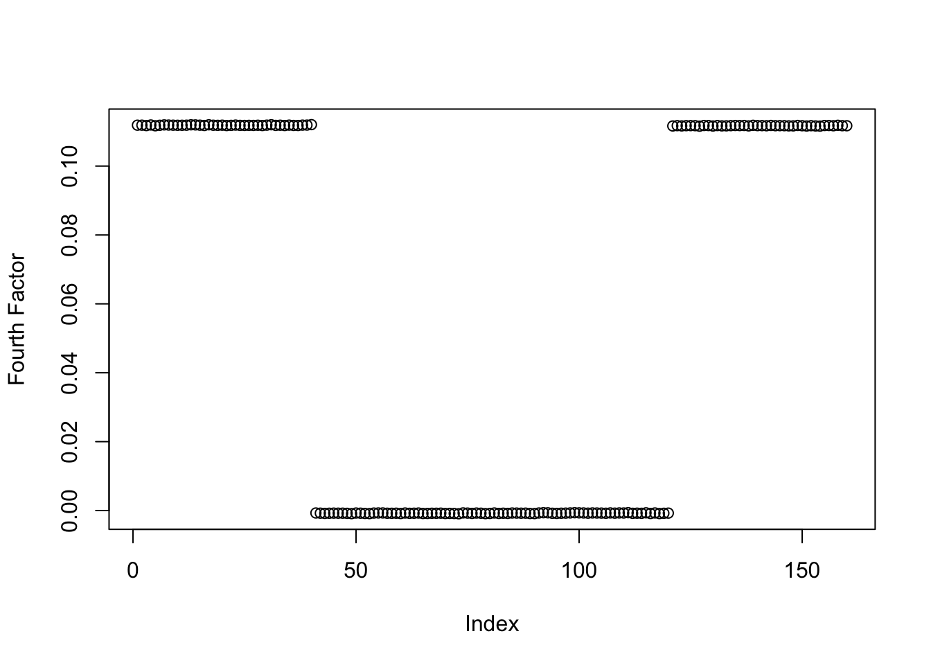
This is the ELBO:
symebcovmf_binormal_fit$elbo[1] -14313.79symEBcovMF with binormal prior finds a similar estimate to that from symEBcovMF with generalized binary prior.
sessionInfo()R version 4.3.2 (2023-10-31)
Platform: aarch64-apple-darwin20 (64-bit)
Running under: macOS Sonoma 14.4.1
Matrix products: default
BLAS: /Library/Frameworks/R.framework/Versions/4.3-arm64/Resources/lib/libRblas.0.dylib
LAPACK: /Library/Frameworks/R.framework/Versions/4.3-arm64/Resources/lib/libRlapack.dylib; LAPACK version 3.11.0
locale:
[1] en_US.UTF-8/en_US.UTF-8/en_US.UTF-8/C/en_US.UTF-8/en_US.UTF-8
time zone: America/Chicago
tzcode source: internal
attached base packages:
[1] stats graphics grDevices utils datasets methods base
other attached packages:
[1] ggplot2_3.5.1 pheatmap_1.0.12 ebnm_1.1-34 workflowr_1.7.1
loaded via a namespace (and not attached):
[1] gtable_0.3.5 xfun_0.48 bslib_0.8.0 processx_3.8.4
[5] lattice_0.22-6 callr_3.7.6 vctrs_0.6.5 tools_4.3.2
[9] ps_1.7.7 generics_0.1.3 tibble_3.2.1 fansi_1.0.6
[13] highr_0.11 pkgconfig_2.0.3 Matrix_1.6-5 SQUAREM_2021.1
[17] RColorBrewer_1.1-3 lifecycle_1.0.4 truncnorm_1.0-9 farver_2.1.2
[21] compiler_4.3.2 stringr_1.5.1 git2r_0.33.0 munsell_0.5.1
[25] getPass_0.2-4 httpuv_1.6.15 htmltools_0.5.8.1 sass_0.4.9
[29] yaml_2.3.10 later_1.3.2 pillar_1.9.0 jquerylib_0.1.4
[33] whisker_0.4.1 cachem_1.1.0 trust_0.1-8 RSpectra_0.16-2
[37] tidyselect_1.2.1 digest_0.6.37 stringi_1.8.4 dplyr_1.1.4
[41] ashr_2.2-66 labeling_0.4.3 splines_4.3.2 rprojroot_2.0.4
[45] fastmap_1.2.0 grid_4.3.2 colorspace_2.1-1 cli_3.6.3
[49] invgamma_1.1 magrittr_2.0.3 utf8_1.2.4 withr_3.0.1
[53] scales_1.3.0 promises_1.3.0 horseshoe_0.2.0 rmarkdown_2.28
[57] httr_1.4.7 deconvolveR_1.2-1 evaluate_1.0.0 knitr_1.48
[61] irlba_2.3.5.1 rlang_1.1.4 Rcpp_1.0.13 mixsqp_0.3-54
[65] glue_1.8.0 rstudioapi_0.16.0 jsonlite_1.8.9 R6_2.5.1
[69] fs_1.6.4